How to visualize a line integral convolution for a vector field with yt
Visualization of Vector Fields
When I was working on my first publication with Prof. Robert Fisher, we explored several ways to visualize the magnetic field in our simulations of white dwarf binary merger. Finally we drew magnetic field in the form of streamlines, which did a satisfactory job. However, since the streamlines could not be arbitrarily dense, the magnetic field geometry was not spatially continuous and the information near pixel scale was lost.
Until recently, I got to know the method of line integral convolution (LIC) and adapted the SciPy cookbook example to yt. The basic idea of LIC is to convolute vector field orientation with local texture over a certain kernel length, thus all the details of vector field geometry can be preserved.
Draw LIC with ONE Line of Code
Drawing LIC for your data with yt is extremely easy – just with a single line of code:
import yt
ds = yt.load("IsolatedGalaxy/galaxy0030/galaxy0030")
s = yt.SlicePlot(ds, 'z', 'density', center='c', width=(20, 'kpc'))
s.annotate_line_integral_convolution('velocity_x', 'velocity_y',
lim=(0.5,0.65))
s.save()
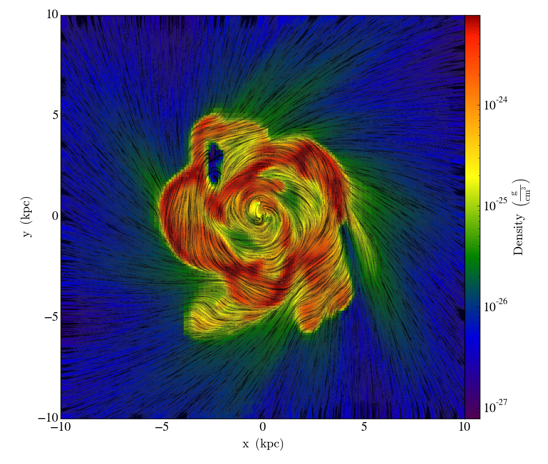
Here velocity_x and velocity_y tell yt to visualize the velocity field, which
is overlaid onto the original density slice plot. Adjusting lim will “squeeze”
the range of LIC magnitude and change the visibility of LIC plot. The code will
produce the following image:

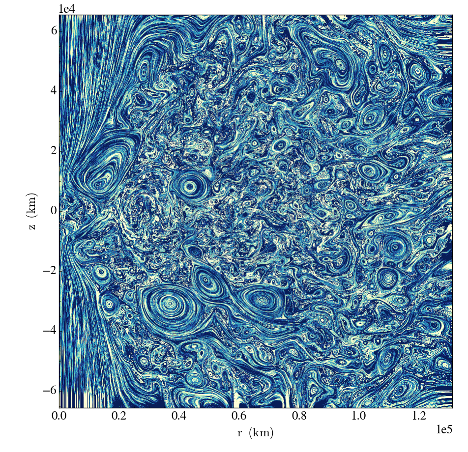
There are more parameters you can play with to generate a perfect image. For instance, although const_alpha is set to False as default to generate a semitransparent LIC image over original plot, you can also set const_alpha to True and use alpha=1 to get a pure LIC image. The following code visualizes LIC of the magnetic field in white dwarf binary simulation:
import yt
ds = yt.load("WDMerger_hdf5_chk_1000/WDMerger_hdf5_chk_1000.hdf5")
s = yt.SlicePlot(ds, 'theta', 'magnetic_field_strength', origin='native')
s.annotate_line_integral_convolution('magnetic_field_x', 'magnetic_field_y',
lim=(0.45,0.55), cmap='YlGnBu', alpha=1.,const_alpha=True)
s.hide_colorbar()
s.save()
and the following image is produced:


