After a significant amount of development and restructuring, I have added the AMR kd-Tree rendering framework to yt. There are several posts on this blog about this module already, so I won’t go over all the background information again. Here I’d like to showcase some of the recent successes and capabilities of the volume rendering within yt.
New optimization options:There are a few important additions that have made it possible to render some of the largest AMR simulations we have available. The first is parallel kd-tree construction. The kd-tree is constructed by first building to the point where there are N kd-Tree nodes. At that point, each processor is assigned a single node to continue building their subtree. This volume decomposes the kd-Tree construction process. If requested, the tree can then be combined through an mpi all-to-all like process.
The next optimization comes in through the type of ray casting. For the largest AMR simulations, it can take time to reduce the kd-Tree once it has been constructed in parallel. To counter this, we have added a ‘domain’ traversal such that each processor only renders it’s subtree. This means that all the data stays local to a processor independent of viewpoint or any other camera parameters. For datasets such as the 512L7 ‘Santa Fe Lightcone’ simulation, this turned out to be very important.
Finally, when the data reading dominates the rendering process, we have added an option in the camera object called no_ghost=True/False. When True, instead of interpolating the vertex centered data from the ghost zones (which requires substantial data reading from neighbors), it extrapolates out to the vertices using the grid’s own data. While less accurate, when using smooth, broad, transfer functions or when just getting an initial look at the data, this provides a substantial speedup.
Showcase examples: For each of these, I am selecting a slice of the volume since there are so many objects. Therefore the depth of each of these are 0.2 in units of the box length.
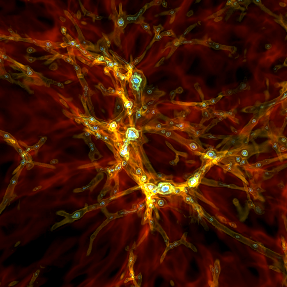
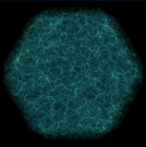
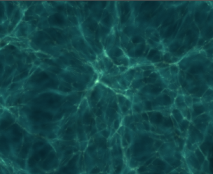
The first example is a 256^3 root grid with 5 levels of AMR, for a total of 48339 grids. Using an 8-core Mac Pro 2.93 GHz desktop, we were able to render a 4096^2 image in just over 100 seconds. kd-Tree construction:21 seconds data reading: 8 secondsray casting: 81 seconds Here is a zoom in of roughly 1/4 of the image:

The second example is a 512^3 root grid + 7 levels of AMR, and is also known as the Santa Fe Lightcone. This simulation has 392,865 grids. For this simulation, we used 256 mpi tasks running on 1024 total cores of TACC Ranger (4way1024). Here the parallel kd-Tree construction really shined, as shown in the timing stats. The image was also 4096^2.
- kd-Tree construction: 6 seconds
- data reading: 100 seconds
- ray casting: 50 seconds
Here are a couple shots, the first showing the entire field of view, and the second showing full resolution in a small portion of the simulation.
I’m pretty happy with the performance and results. Since the data doesn’t have to be moved around in between frames, I’m hoping to make some great movies of these large datasets exploring the rich interactions and features that are undoubtably hiding in the data.
If you give this new renderer a shot and have any impressions or questions, let me know!


