Matthew Turk 0000-0002-5294-0198
· MatthewTurk
· powersoffour
School of Information Sciences, University of Illinois at Urbana-Champaign; Department of Astronomy, University of Illinois at Urbana-Champaign
Nathan J Goldbaum 0000-0001-5557-267X
· ngoldbaum
· njgoldbaum
National Center for Supercomputing Applications, University of Illinois at Urbana-Champaign
Jared W. Coughlin 0000-0002-4373-4114
· jcoughlin11
National Center for Supercomputing Applications, University of Illinois at Urbana-Champaign
Corentin Cadiou 0000-0003-2285-0332
· cphyc
· cphyc
Department of Physics and Astrophysics, University College London; Institut d’Astrophysique de Paris
We present the current version of the yt software package.
yt is an open-source, community-developed platform for analysis of volumetric data, with readers for several dozen data formats, indexing systems for gridded data, adaptive mesh refinement data, unstructured mesh data, discrete and particle formats, and octree-based data, as well as the combination of these.
We describe the systems implemented in yt to facilitate a “science-first” approach to data analysis, wherein the emphasis is on the meaning and interpretation of the data as opposed to its discretization or layout.
Authorship Policy
We note that the author list for this paper is, by design, extensive.
We have separated the authors into those that contributed to the text (whose names are ordered somehow TBD) and those that are members of the yt community.
The authors from each group have been indicated in the respective author affiliations.
This paper was developed collaboratively, using the Manubot [1] system for collaborating on and reviewing contributed text.
To add yourself to the author list, please follow the instructions in our
README.
Introduction
The process of transforming data into understanding constitutes the vast majority of time, energy, and intellectual effort spent during scientific inquiry.
This is true across domains, whether data is the product of a computational simulation, a telescope observation, the synthesis of sensors distributed across the Earth, or a collection of images of the human brain.
Data, by themselves, do not reflect an understanding of the Universe or its underlying physical properties; rather, they are recordings, or measurements, of the state of systems as observed.
Even for computational simulations, such as simulations of star formation in the galaxy, this is true: these simulations encode information about a discretization of a model, rather than the model itself.
Bridging the gap between this discretization and the physical understanding requires accessing data, manipulating and interrogating this data, and then applying to this data a sense of understanding.
Somehow, bits stored on a disk must become, in our minds, a galaxy undergoing a starburst.
This process is both mediated and impeded by computational tools.
When those tools align with our mental model of how data exists, they can allow us to work more efficiently, asking questions of data and building sophisticated scientific inquiry.
However, when they do not, they can cause frustration, delays, and most worryingly, incorrect or misinterpreted results.
When viewing this from the perspective of the landscape of inquiry, the most startling realization is that the questions a computational tool enables individuals to ask shapes the questions they think to ask.
In [2], the analysis platform yt was described.
At the time, yt was focused on analyzing and visualizing the output of grid-based adaptive mesh refinement hydrodynamic simulations; while these were used to study many different physical phenomena, they all were laid out in roughly the same way, in rectilinear meshes of data.
In this paper, we present the current version of yt, which enables identical scripts to analyze and visualize data stored as rectilinear grids as before, but additionally particle or discrete data, octree-based data, and data stored as unstructured meshes.
This has been the result of a large-scale effort to rewrite the underlying machinery within yt for accessing data, indexing that data, and providing it in efficient ways to higher-level routines, as discussed in Section Something.
While this was underway, yt has also been considerably reinstrumented with metadata-aware array infrastructure, the volume rendering infrastructure has been rewritten to be more user-friendly and capable, and support for non-Cartesian geometries has been added.
The single biggest change to yt since that paper was published has not been technical in nature.
In the intervening years, a directed and intense community-building effort has resulted in the contributions from over a hundred different individuals, many of them early-stage researchers, and a thriving community of both users and developers.
This is the crowning achievement of development, as we have attempted to build yt into a tool that enables inquiry from a technical level as well as fosters a supportive, friendly community of individuals engaged in self-directed inquiry.
Community Building
Choosing a software package for a particular purpose involves evaluating several differentiating factors; these factors include the functionality of a package, the performance of a package, the user-friendliness, and even the ability of an individual to find help, engage with others and feel a sense of participation.
cite something here The development, fostering and design of the community around yt is deemed to be both crucial to the success or failure of yt, and in many ways inseparable from its functionality.
Composition
There are several rough categories of individuals engaged in development and utilization of yt.
As a result of its API-first design, there are few if any individuals who use yt that do not do so through the scripting interface; this means that the vast (if not exclusive) majority of individuals who interact with the functionality in yt are doing so by writing their own scripts, modules, and code, and arguably engaging in a value-added development process of their own.
The majority of individuals using yt at present are in astronomy and astrophysics, typically fields of simulation, although representatives from other domains are increasingly participating in development and using yt for their own domain-specific problems
Making the distinction somewhat more clearly, there are individuals who have built their own scripts and utilized them as well as individuals who have contributed changes or modules to the primary yt codebase.
In addition, there is an emerging set of projects that build on yt as infrastructure to conduct scientific analysis.
These developers are largely driven by their own pragmatic scientific needs, and they constitute the majority of developers (by number) that contribute to the code base.
The majority of these individuals are early- to mid-career researchers, typically graduate students, postdocs, and assistant professors.
In recent years, there has emerged a more coherent contingency of individuals who participate in both pragmatically-focused development of modules and functionality for their own benefit as well as modules or overall improvement that is supplemental or even external to their own research agenda.
Sections of the code base receiving such improvements include unit handling, plotting code, infrastructure for loading disparate datasets, and so on.
At this time we do not know of any individuals funded to work on yt completely independent of a scientific or scholarly goal.
The composition of the community, particularly with a mixture of timelines for goal-setting and completion, can at times cause frustrations and difficulties.
For instance, the response to “Can this feature be implemented?” often includes an invitation for the questioner to collaborate on developing that feature and submitting it to the codebase.
Developing a schedule of releases is an act of consensus building, both deciding what bugs are critical to fix in the timeline of a release as well as building consensus on what features should be considered blockers for a new release.
The intersection of this with academic deadlines (for instance job application season) requires balance and care.
Types of Tasks
When evaluating the level of engagement, we consider a few different classifications of tasks that are performed by individuals in the community, and evaluate these based on how they flow into greater engagement.
Filing issues
Participating in mailing list discussions
Issuing a pull request
Writing documentation
Participating in code review
Drafting an enhancement proposal
Closing bug reports
While there are other activities that individuals can participate in, these are the typical activities we see among participants in the community.
The order, flowing from the first to the last, is the typical flow we see for an individual coming to participate in the community.
The first step is typically to file an issue or bug report (occasionally these are requests for new features), followed by participating in development-focused discussion on mailing lists.
The next level of engagement typically involves the development of a new piece of functionality, refinement of existing code, or issuing a fix for a bug or issue.
These take the form of pull requests (described in greater detail here) that can be reviewed and added to the code base.
The next level of engagement centers around tasks that are not fully-aligned with pragmatic, code-driven scientific inquiry.
The development of documentation is often viewed as orthogonal to the scientific process, and typically requires an iterative writing process.
Participation in code review, providing comments, feedback and suggestions to other authors, is another somewhat orthogonal task; it doesn’t necessarily directly benefit the developer doing the reviewing (although it might) and it does not necessarily result in academic rewards (citations, authorship, etc).
But, it does arise from a pragmatic (ensuring code reliability) or altruistic (the public good of the software) motivation, and is thus a deeper level of engagement.
The final two activities, drafting enhancement proposals and closing bug reports, are the most engaged, and often the most removed from the academic motivation structure.
Developing an enhancement proposal for yt means iterating with other developers on the motivation behind and implementation of a large piece of functionality; it requires both motivation to engage with the community and the patience to build consensus among stakeholders.
Closing bug reports – and the development work associated with identifying, tracking and fixing bugs – requires patience and often repeated engagement with stakeholders.
Engagement Metrics
We include here plots of the level of engagement on mailing list discussions and the citation count of the original method paper.
Governance
Between the publication of the first paper and this paper, the yt project instituted a form of governance involving a steering committee, a set of “members” of the project, and a defined process for developing improvements and enhancements (the YTEP, or yt-enhancement-proposal process).
YTEPs are discussed in [sec:ytep].
The systems developed account for a number of important procedures, mostly related to decision-making, but do not address pressing community needs such as community standards for conduct, changes in committee composition, sub-project coordination, or the transition of members and developers to “emeritus” status.
Development Procedure
yt is developed openly.
During the Spring of 2017, development transitioned from occurring on Bitbucket to GitHub, and the source code management system was changed from Mercurial to git.
Development occurs through the “pull request” model, wherein changes to the codebase are made and then requested to be included in the primary repository.
Typically, there are two branches of development, and occasionally three. The first of these is the “stable” branch, which is much slower-paced, and typically only modified during the release periods.
The second is that of “main” (formerly “master”, which is the conventional term in git terminology, and renamed in early 2021; the corresponding mercurial term would be “default”) which is where current development takes place.
The “main” branch is meant to be for development proceeding that does not drastically disrupt usage patterns.
Occasionally, such as during the development of yt 4.0, a third branch is included in the primary repository.
This development branch is open for large and potentially disruptive changes, but in order to centralize code review and developer attention it takes place there.
For instance, during the development of yt 4.0, the branch yt-4.0 was where the global mesh was removed and where the units subsystem was removed and replaced with unyt.
This three-pronged approach generally has suited the community; the process of backporting changes from the “main” branch to the “stable” branch can be time-consuming.
However, balancing the needs of a community requiring stable methods for analyzing data against the ease of development suggests that this is a toll worth paying.
In general, the development of yt is reasonably top-heavy, with the majority of contributions coming from a core group of individuals.
We discuss the implications of this on sustainability in Section [sec:sustainability].
Unit Testing
The yt codebase includes a number of unit tests; although extensive, their existence post-dates the initial development of the code, and they largely work around the extant APIs at the time of their creation.
Most modern recommendations for developing scientific software emphasize isolated components, well-structured interfaces, and few side effects.
While the development process attempts to emphasize development of isolated APIs and well-constrained unit tests, the balance struck between enabling contribution from junior developers and ensuring the (subjective) standards of the code base does not always fall on the side of rigid design.
Many of the yt APIs that are tested require the existence of a “dataset.”
For instance, the testing of whether objects are correctly selected by a sphere selector (which absolutely could be tested in isolation, were the APIs more separable) is done via creating several different sets of mock datasets of different organizations and shapes and testing whether or not they correctly choose the data points to be included.
To support these operations, the yt testing utilities provide helper functions for creating mock datasets that have different geometric configurations and different collections of “fields” included in their set of primitive values.
Many of the tests are parameterized against the types and organizations of the datasets, the decomposition across mock processors, and the underlying values of the fields.
This ensures that we check against errors and bugs that may depend on behavior that varies as the number of processors or the organization of the data changes.
One example of this would be in the selection of grid values for a single grid of size \(128^3\).
The values selected in this should match the values selected in the same grid decomposed into eight sets of \(64^3\) cells, or 64 sets of \(32^3\) cells.
The mechanism by which fields are tested is somewhat more extensive, touching on two different needs.
The first need is that of accuracy – fields with known answers, or fields that can be written to be decomposed into primitive, non-optimized operations, are tested for correctness.
The second need is that of dependency calculation; all fields should have their dependencies correctly detected.
For example, if a dataset has primitive fields for “mass” and “velocity,” the calculation of momentum should require both.
If the dataset includes a “momentum” field, then that should be detected as well.
This dependency calculation enables yt to consolidate IO tasks and read as much data as possible in each pass over the full dataset.
In addition to this, fields are tested to ensure that the values generated for them are independent of the organization of the dataset.
Like in the example above, the “momentum” field for a fixed set of values should be identical regardless of the decomposition of the individual cell elements.
Wherever possible, analytical solutions are preferred.
For processes like surface extraction, this might include ensuring that fixed radii extraction produce the correct spherical region.
For streamlines, it might include computing the analytical solution to an integration along a known vector field.
And for projections, it would mean that integrating the path with a weight of “one” should result in a uniform set of values equal to the path length across the domain.
At present, the unit tests in yt take a considerable amount of time to run, and are using the nosetests framework. Modern Python practice is to use the newer pytest framework, and efforts are underway to port yt to utilize pytest, and in the process, attempt to reduce overall runtime.
Answer Testing
The most time-consuming part of the testing process is what we refer to as “answer testing.”
Because so much of yt is focused on computing analysis results, and because some of these analysis results simultaneously depend on specific IO routines, selection routines, and many “frontend-specific” pieces of code, we have built a system for ensuring that for a given set of analysis operations, the result of a set of operations does not change beyond a fixed (typically quite small) tolerance.
Code Review
Code review in yt is conducted on a line-by-line basis, as well as on a higher-level regarding pull requests.
The workflow for code review roughly follows this outline:
A pull request is issued. When a new pull request is issued, a template is provided that includes a description of the change, requesting information about its compliance with coding standards, etc.
The pull request is automatically marked as unmergeable until a team member applies the correct component label.
Code is reviewed, line-by-line, and suggestions are made by humans. Code linting is automated.
This process is iterated, ensuring that tests, results accuracy and coding standards are maintained.
One increasing issue with the code review process is ensuring that changes are reviewed with appropriate urgency; larger pull requests tend to languish without review, as the requirements for review necessarily add burden to the maintainers.
“Bugfix” changes formally require only one reviewer, whereas the yt guidelines suggest that larger changes require review from two different team members.
YTEP Process
YTEPs, or “yt-enhancement proposal” are vehicles for collaborative decision-making in the project.
Implemented shortly after the first paper on yt was released, the YTEP process experienced a fairly pronounced period of usage during the transition between versions 2.0 and 3.0 of yt, and has since been utilized considerably less.
During periods of rapid development, the needs of the community for stability have to be balanced against desires for change; the YTEP process was implemented to facilitate stakeholder feedback, allow for discussion of design decisions, and to prompt detailed thinking about how and why things should be implemented.
We have modeled this process against that used in the AstroPy community (“APE”).
To create a new proposal for a large change to yt, or to document a decision-making process, individuals prepare a description of the background, motivation for the change, the steps to implementation, and potential alternative approaches.
The proposal is discussed through the pull-request process, and once discussion has concluded it is added to the repository of YTEPs that is auto-built and deployed.
The accepted YTEPs have included implementing the chunking system, developing a units system, removing legacy components, and implementing a code of conduct.
Below, we include a table of current YTEPs as of this writing.
Number
YTEP Title
Created
Authors
0001
IO Chunking
November 26, 2012
Matthew Turk
0002
Profile Plotter
December 5, 2012
Matthew Turk
0003
Standardizing field names
December 11, 2012
Casey Stark, Nathan Goldbaum, Matthew Turk
0005
Octrees for Fluids and Particles
December 24, 2012
Matthew Turk
0006
Periodicity
January 10, 2013
Matthew Turk, Nathan Goldbaum
0007
Automatic Pull Requests’ validation
February 21, 2013
Kacper Kowalik
0008
Release Schedule
February 21, 2013
Matthew Turk
0009
AMRKDTree for Data Sources
February 28, 2012
Sam Skillman
0010
Refactoring for Volume Rendering and Movie Generation
March 3, 2013
Cameron Hummels
0011
Symbol units in yt
March 7, 2013
Nathan Goldbaum, Casey Stark, Anna Rosen, Matthew Turk
0012
Halo Redesign
March 7, 2013
Britton Smith, Cameron Hummels, Chris Moody, Mark Richardson, Yu Lu
0013
Deposited Particle Fields
April 25, 2013
Chris Moody, Matthew Turk, Britton Smith, Doug Rudd, Sam Leitner
0014
Field Filters
July 2nd, 2013
Matthew Turk
0015
Transfer Function Refactor
August 13, 2013
Sam Skillman
0016
Volume Traversal
September 10, 2013
Matthew Turk
0017
Domain-Specific Output Types
September 18, 2013
Matthew Turk and Anthony Scopatz
0018
Changing dict-like access to Static Output
September 18, 2013
Matthew Turk
0019
Reduce items in main import
October 2, 2013
Matthew Turk
0020
Removing PlotCollection
March 18, 2014
Matthew Turk
0021
Particle-Only Plots
August 29, 2014
Andrew Myers
0022
Benchmarks
January 19, 2015
Matthew Turk
0023
yt Community Code of Conduct
July 11, 2015
Britton Smith
0024
Alternative Smoothing Kernels
August 1, 2015
Bili Dong
0025
The ytdata Frontend
August 31, 2015
Britton Smith
0026
NumPy-like Operations
September 21, 2015
Matthew Turk
0027
Non-Spatial Data
December 1, 2015
Matthew Turk, Nathan Goldbaum, John ZuHone
0028
Alternative Unit Systems
December 8, 2015
John ZuHone, Nathan Goldbaum, Matthew Turk
0029
Extension Packages
January 25, 2016
Matthew Turk
0031
Unstructured Mesh
December 18, 2014
Matthew Turk
0032
Removing the global octree mesh for particle data
February 9 2017
Nathan Goldbaum, Meagan Lang, Matthew Turk
0033
Dropping Python2 Support
November 28, 2017
Nathan Goldbaum
0034
yt FITS Image Standard
September 9, 2018
John ZuHone
0036
Migrating from nose to pytest
September 30, 2019
Jared Coughlin
0037
Code Styling
May 18, 2020
Clément Robert
1000
GitHub Migration
March 25, 2017
Lots of folks
1776
Team Infrastructure
August 24, 2014
Britton Smith
3000
Let’s all start using yt 3.0!
October 30, 2013
Matthew Turk
Indexing and Geometry
yt is designed for analysis and visualization of datasets that describe “natural” or “physical” phenomena; more generally, yt is designed to analyze data that can be characterized by a metric of some type.
The most common use case, by far, is that of data that is described in a Cartesian space, by the orthogonal axes of x, y and z.
However, for reasons related to naturalness of coordinate systems and relevance to physical phenomena, datasets are also frequently organized in other coordinate systems, such as cylindrical polar (\(r\), \(z\) and \(\theta\)), spherical (\(r\), \(\theta\) and \(\phi\)) and variants such as geographic (latitude, longitude and altitude).
Importantly, however, yt distinguishes between the coordinate space a dataset describes and the natural or index space by which its organization is described.
This distinction is the most relevant among datasets and data formats where the organization is implicit, rather than explicit; for instance, in a grid patch dataset, data variable locations are often only specified implicitly.
For a grid volume that covers a given region, the relationship between the “index” value of a cell (for instance, \(i,j,k\)) and its position in space (for instance, \(x, y, z\) or \(r, \theta, \phi\)) requires transformation between a logically-Cartesian decomposition of the space and the potentially-non Cartesian space that it represents.
In Figure 1 we demonstrate one possible mapping.
We note that the specific data layout is not optimized for IO throughput, and is unlikely to be exactly replicated in real world formats.
In this case, the data points may be laid out sequentially on disk (or in memory) and a mapping function translates these into position and extent in the coordinate system, here cylindrical coordinates.
For instance, there may be a cell that spans \(r\) from 0.375 to 0.5 and
\(\theta\) from 45.0 to 52.5, which is defined by the array values defined in cell 1, 4.
Figure 1: Index space to coordinate space mapping. On the left is an example of how data points may be laid out on disk and on the right is how these points might be translated into a (cylindrical) coordinate space.
Abstraction of Coordinate Systems
yt provides a system for defining relationships between index-space and coordinate-space.
During instantiation of a Dataset object, a helper object (coordinates, a subclass of CoordinateHandler) is created.
This helper object tracks the correspondence between numerical axes and spatial axes (for instance, even in some Cartesian datasets, axis 0 corresponds to \(z\) rather than \(x\)), the names of axes, and the transformation and pixelization methods for visualization.
In addition to these helper functions, the coordinate handler provides definitions for derived fields that describe local cell width (and orthogonal path length), positions in coordinate space as computed by index space coordinates, volumes, and surface areas.
These coordinate handlers also provide transformations between different spaces, albeit using the somewhat undesirable method of conversion to reference cartesian frames and subsequent conversion to local coordinate frames.
At present, coordinate spaces are defined in the spaces enumerate in Table 1.
While these are representative of the most common spatial representations, additional representations (such as those that include a non-trivial mapping between coordinates and index values) are possible to implement.
Table 1: Extant coordinate systems; in all cases, value ranges should be taken to describe extent rather than specific boundary points.
Coordinate system
Axes
Cartesian coordinates
\(x, y, z\)
Cylindrical polar coordinates
\(r, \theta \in [0, 2 \pi], z\)
Spherical coordinates
\(r, \theta, \phi\)
Geographic coordinates
latitude \(\in [0, 180]\), longitude \(\in [0, 360]\), altitude
Internal geographic coordinates
latitude, longitude, depth
Spectral cube
Image \(x\), Image \(y\) and \(\nu\)
Future developments may involve code generation for arbitrary coordinate systems, using SymPy or other libraries.
Independent of the visualization methods (which can often be reused), the development of coordinate systems is largely rote, applying straightforward mathematics to construct derived field definitions.
As such, using mechanisms in SymPy for construction of relationships between coordinate systems may be a feasible method of developing code-generation for coordinate system handlers in yt.
Data Objects
The basic principles by which yt operates are built on the notion of selecting data (through coarse and subsequent fine-grained indexing of data sources such as files), accessing that data in a memory-efficient fashion, and then processing that data into either a resultant set of quantitative data or a visualization.
Selections in yt are usually spatial in nature, although several non-spatial mechanisms focused on queries can be utilized as well.
These objects which conduct selection are selectors, and are designed to provide as small of an API as possible, to enable ease of development and deployment of new selectors.
Selectors require defining several functions, with the option of defining additional functions for optimization, that return true or false whether a given point is or is not included in the selected region.
These functions include selection of a rectilinear grid (or any point within that grid), selection of a point with zero extent and selection of a point with a non-zero spherical radius.
The base selector object utilizes these routines during a selection operation to maximize the amount of code reused between particle, patch, and octree selection of data.
These three types of data are selected through specific routines designed to minimize the number of times that the selection function must be called, as they can be quite expensive.
Selecting data from a grid is a two-step process.
The first step is identifying which grids intersect a given data selector; this is done through a sequence of bounding box intersection checks.
Within a given grid, the cells which are intersected are identified.
This results in the selection routine being called once for each grid object in the simulation and once for each cell located within an intersecting grid.
This can be conducted hierarchically, but due to implementation details around how the grid index is stored this is not yet cost effective.
Selecting data from an octree-organized dataset utilizes a recursive scheme that selects individual oct nodes, then for each cell within that oct, determining which cells must be selected or child nodes recursed into.
This system is designed to allow for having leaf nodes of varying cells-per-side, for instance 1, 2, 4, 8, etc.
However, the number of nodes is fixed at 8, with subdivision always occurring at the midplane.
The final mechanism by which data is selected is for discrete data points, typically particles in astrophysical simulations.
At present, this is done by first identifying which data files intersect with a given selector, then selecting individual points.
There is no hierarchical data selection conducted in this system, as we do not yet allow for re-ordering of data on disk or in-memory which would facilitate hierarchical selection through the use of operations such as Morton indices.
Selection Routines
Given these set of hierarchical selection methods, all of which are designed to provide opportunities for early-termination, each geometric selector object is required to implement a small set of methods to expose its functionality to the hierarchical selection process.
Duplicative functions often result from attempts to avoid expensive calculations that take into account boundary conditions such as periodicity and reflectivity unless necessary.
Additionally, by providing some routines as options, we can in some instances specialize them for the specific geometric operation.
select_cell(cell_center, cell_width): this function, which is somewhat degenerate with select_bbox, returns whether a given “cell,” defined by its center and its width along each dimension, is included within the selection. In situations where the cells are spaced logarithmically, rather than linearly, this may produce slightly reduced accuracy for near-misses and glancing-selections.
select_point(position): this function returns whether or not a point of zero-extent is included within the selection. This has some degeneracy with select_sphere.
select_sphere(position, radius): This is equivalent to the select_point function, except that any point within the specified radius is included within the selector object.
select_bbox(lower_left, upper_right): Determine overlap with an axis-aligned bounding box. Particularly for hierarchical selection methods, determining whether or not a bounding box overlaps with a geometric selector can lead to early-termination of some selection operations.
select_bbox_edge(lower_left, upper_right): This is a special-case of the bounding box routine that provides information as to whether or not the entire bounding box is included or just a partial portion of the bounding box.
We demonstrate a handful of selection operations on a low-resolution dataset below.
In Figure 2 we illustrate the selection of a rectangular prism (i.e., a region, like in Section [sec:dobj-region].
In Figure 3, we illustrate the selection of a sphere (i.e., a sphere, like in Section [sec:dobj-sphere].
And, to demonstrate yt’s ability to construct boolean selectors from these objects (i.e., Section [sec:dobj-bool] we show what the logical NOT of these two objects would produce in 4.
Figure 2: A selection of data in a low-resolution simulation from a rectangular prism.
Figure 3: A selection of data in a low-resolution simulation from a sphere.
Figure 4: The logical A AND NOT B for regions A and B from Figures 2 and 3 respectively.
Fast and Slow Paths
Given an ensemble of objects, the simplest way of testing for inclusion in a selector is to call the operation select_cell on each individual object.
Where the objects are organized in a regular fashion, for instance a “grid” that contains many “cells,” we can apply both “first pass” and “second pass” fast-path operations.
The “first pass” checks whether or not the given ensemble of objects is included, and only iterates inward if there is partial or total inclusion.
The “second pass” fast pass is specialized to both the organization of the objects and the selector itself, and is used to determine whether either only a specific (and well-defined) subset of the objects is included or the entirety of them.
For instance, we can examine the specific case of selecting grid cells within a rectangular prism.
When we select a “grid” of cells within a rectangular prism, we can have either total inclusion, partial inclusion, or full exclusion.
In the case of full inclusion, where the entire grid is included within the selector, we simply sidestep the specific inclusion checks completely and return a full mask of cells to utilize.
In the case of partial inclusion, we can often determine the “start” and “end” indices of inclusion in the rectangular prism by examining the intersection volume.
This allows us to avoid many costly individual select_cell calls.
With discrete point selection (and for our purposes, often unstructured mesh falls into this category) we often do not have the same organizing principle on which we can rely.
However, utilizing hierarchical bitmap indexing we can often organize subsets of particles into collections of cells which may or may not be contiguous.
In this situation, we can check for full inclusion within data objects, although we are not able to identify start and stop indices as the data are not assumed to be organized spatially independent of how we have indexed them.
At present, the objects listed in 2 are provided as selectors in yt.
We do make a distinction between “selection” operations and “reduction” or “construction” operations (such as projections and smoothing/resampling), but have included both here for consistency.
Additionally, some have been marked as not “user-facing,” in the sense that they are not expected to be constructed directly by users, but instead are utilized internally for indexing purposes.
In columns to the right, we provide information as to whether there is an available “fast” path for grid objects.
Table 2: Selection objects and their types.
Object Name
Object Type
Arbitrary grid
Resampling
Boolean object
Selection (Base Class)
Covering grid
Resampling
Cut region
Selection
Cutting plane
Selection
Data collection
Selection
Disk
Selection
Ellipsoid
Selection
Intersection
Selection (Bool)
Octree
Internal index
Orthogonal ray
Selection
Particle projection
Reduction
Point
Selection
Quadtree projection
Reduction
Ray
Selection
Rectangular Prism
Selection
Slice
Selection
Smoothed covering grid
Resampling
Sphere
Selection
Streamline
Selection
Surface
Selection
Union
Selection (Bool)
Arbitrary grid
Arguments:
Left edge
Right edge
Active Dimensions
A 3D region with arbitrary bounds and dimensions. In contrast to the
Covering Grid, this object accepts a left edge, a right edge, and
dimensions. This allows it to be used for creating 3D particle
deposition fields that are independent of the underlying mesh, whether
that is yt-generated or from the simulation data. For example,
arbitrary boxes around particles can be drawn and particle deposition
fields can be created. This object will refuse to generate any fluid
fields.
Bool
Arguments:
Operation
Data object 1
Data object 2
This is a boolean operation, accepting AND, OR, XOR, and NOT for
combining multiple data objects. This object is not designed to be
created directly; it is designed to be created implicitly by using one
of the bitwise operations (&, |, ^, ~) on one or two other data
objects. These correspond to the appropriate boolean operations, and
the resultant object can be nested.
Covering grid
Arguments:
Level
Left edge
Active Dimensions
A 3D region with all data extracted to a single, specified resolution.
Left edge should align with a cell boundary, but defaults to the
closest cell boundary.
Cut region
Arguments:
Base object
Conditionals
This is a data object designed to allow individuals to apply logical
operations to fields and filter as a result of those cuts.
Cutting
Arguments:
Normal
Center
This is a data object corresponding to an oblique slice through the
simulation domain. This object is typically accessed through the
cutting object that hangs off of index objects. A cutting plane is
an oblique plane through the data, defined by a normal vector and a
coordinate. It attempts to guess an ‘north’ vector, which can be
overridden, and then it pixelizes the appropriate data onto the plane
without interpolation.
Data collection
Arguments:
Object List
By selecting an arbitrary object_list, we can act on those grids.
Child cells are not returned.
Disk
Arguments:
Center
Normal vector
Radius
Height
By providing a center, a normal, a radius and a height we can
define a cylinder of any proportion. Only cells whose centers are
within the cylinder will be selected.
Ellipsoid
Arguments:
Center
a
b
c
e0
tilt
By providing a center,A,B,C,e0,tilt we can define a
ellipsoid of any proportion. Only cells whose centers are within the
ellipsoid will be selected.
Intersection
Arguments:
Data objects
This is a more efficient method of selecting the intersection of
multiple data selection objects. Creating one of these objects
returns the intersection of all of the sub-objects; it is designed to
be a faster method than chaining & (“and”) operations to create a
single, large intersection.
Minimal sphere
Arguments:
Center
Radius
Build the smallest sphere that encompasses a set of points.
Octree
Arguments:
Left edge
Right edge
Particle count refinement criteria
A 3D region with all the data filled into an octree. This container
will mean deposit particle fields onto octs using a kernel and SPH
smoothing.
Ortho ray
Arguments:
Axis
Coords
This is an orthogonal ray cast through the entire domain, at a
specific coordinate. This object is typically accessed through the
ortho_ray object that hangs off of index objects. The resulting
arrays have their dimensionality reduced to one, and an ordered list
of points at an (x,y) tuple along axis are available.
Particle proj
Arguments:
Axis
Field
Weight field
A projection operation optimized for SPH particle data.
Point
Arguments:
P
A 0-dimensional object defined by a single point
Quad proj
Arguments:
Axis
Field
Weight field
This is a data object corresponding to a line integral through the
simulation domain. This object is typically accessed through the
proj object that hangs off of index objects. YTQuadTreeProj is a
projection of a field along an axis. The field can have an
associated weight_field, in which case the values are multiplied by
a weight before being summed, and then divided by the sum of that
weight; the two fundamental modes of operating are direct line
integral (no weighting) and average along a line of sight (weighting.)
What makes proj different from the standard projection mechanism is
that it utilizes a quadtree data structure, rather than the old
mechanism for projections. It will not run in parallel, but serial
runs should be substantially faster. Note also that lines of sight
are integrated at every projected finest-level cell.
Ray
Arguments:
Start point
End point
This is an arbitrarily-aligned ray cast through the entire domain, at
a specific coordinate. This object is typically accessed through the
ray object that hangs off of index objects. The resulting arrays
have their dimensionality reduced to one, and an ordered list of
points at an (x,y) tuple along axis are available, as is the t
field, which corresponds to a unitless measurement along the ray from
start to end.
Region
Arguments:
Center
Left edge
Right edge
A 3D region of data with an arbitrary center. Takes an array of three
left_edge coordinates, three right_edge coordinates, and a
center that can be anywhere in the domain. If the selected region
extends past the edges of the domain, no data will be found there,
though the object’s left_edge or right_edge are not modified.
Slice
Arguments:
Axis
Coord
This is a data object corresponding to a slice through the simulation
domain. This object is typically accessed through the slice object
that hangs off of index objects. Slice is an orthogonal slice through
the data, taking all the points at the finest resolution available and
then indexing them. It is more appropriately thought of as a slice
‘operator’ than an object, however, as its field and coordinate can
both change.
Smoothed covering grid
Arguments:
Level
Left edge
Active Dimensions
A 3D region with all data extracted and interpolated to a single,
specified resolution. (Identical to covering_grid, except that it
interpolates.) Smoothed covering grids start at level 0,
interpolating to fill the region to level 1, replacing any cells
actually covered by level 1 data, and then recursively repeating this
process until it reaches the specified level.
Sphere
Arguments:
Center
Radius
A sphere of points defined by a center and a radius.
Streamline
Arguments:
Positions
This is a streamline, which is a set of points defined as being
parallel to some vector field. This object is typically accessed
through the Streamlines.path function. The resulting arrays have
their dimensionality reduced to one, and an ordered list of points at
an (x,y) tuple along axis are available, as is the t field, which
corresponds to a unitless measurement along the ray from start to end.
Surface
Arguments:
Data source
Surface field
Field value
This surface object identifies isocontours on a cell-by-cell basis,
with no consideration of global connectedness, and returns the
vertices of the Triangles in that isocontour. This object simply
returns the vertices of all the triangles calculated by the marching cubes <https://en.wikipedia.org/wiki/Marching_cubes>_ algorithm; for
more complex operations, such as identifying connected sets of cells
above a given threshold, see the extract_connected_sets function.
This is more useful for calculating, for instance, total isocontour
area, or visualizing in an external program (such as MeshLab <http://www.meshlab.net>_.) The object has the properties .vertices
and will sample values if a field is requested. The values are
interpolated to the center of a given face.
Union
Arguments:
Data objects
This is a more efficient method of selecting the union of multiple
data selection objects. Creating one of these objects returns the
union of all of the sub-objects; it is designed to be a faster method
than chaining | (or) operations to create a single, large union.
Processing and Analysis of Data
Array-like Operations
In yt, a newly-constructed data selector contains no data – this enables data selectors for large regions, in extremely large datasets, to be lightweight and cheap to construct.
By ensuring that these objects don’t immediately consume resources, they can be manipulated and operated on in a high-level fashion, without taxing the computational power.
While these data objects can return the full set of data they include, yt also provides array-like operations that do not require immediate access to the full set of numerical values, and which align with the mental-model for data processing that yt exposes.
As an example, consider the following two operations:
dd = ds.all_data()dd["gas", "density"].max()
and
dd = ds.all_data()dd.max(("gas", "density"))
Both are available in yt.
As a side-effect of Python’s object model, the first will access the ("gas", "density") item in the object dd, itself a concatenated numpy array, and then execute the max method on it.
The second will call the max method on the data object, supplying to it the name of the field.
This allows yt to decide how to decompose, parallelize and process the data in a memory-efficient way, and spread across multiple processors.
Additionally, by emphasizing that the “maximum” is being taken on the data object, rather than the numerical data, other operations can be exposed that build on the underlying data organization.
For instance, taking the maximum along a given (spatial) axis:
This translates our meaning – find the maximum value along the z-axis – into a dimensionality reduction operation that uses yt’s built-in “projection” method.
These operations, on data objects (rather than the underlying arrays of values that are accessible through them) provide dataframe-like methods for querying very large, spatially registered data.
The array-like operations utilized in yt attempt to map to conceptually similar operations in numpy.
Unlike numpy, however, these utilize yt’s dataset-aware “chunking” operations, in a manner philosophically similar to the chunking operations used in dask.
Below, we outline the three classes of operations that are available, based on the type of their return value.
Reduction to Scalars
Traditional array operations that map from an array to a scalar are accessible utilizing familiar syntax. These include:
min(field_specification), max(field_specification), and ptp(field_specification)
argmin(field_specification, axis), and argmax(field_specification, axis)
mean(field_specification, weight), std(field_specification, weight), and sum(field_specification)
In addition to the advantages of allowing the parallelism and memory management be handled by yt, these operations are also able to accept multiple fields.
This allows multiple fields to be queried in a single pass over the data, rather than multiple passes.
Additionally, the min and max operations will automatically cache the results during a single pass, which means that calling max immediately after min (and vice versa) on the same data object and field will not require a recomputation.
In the case of argmin and argmax, the default returned “axis” will be the spatial coordinates of the minimum or maximum field value (respectively).
However, by specifying an axis or set of axes that correspond to fields, the field values will be queried at these minimum or maximum points.
This allows, for instance, to query the value of “density” at the minimum “temperature.”
The operations mean and sum are available here in a non-spatial form, where they simply compute the scalar reduction independent of the spatial registration of the dataset.
Reduction to Vectors
profile(axes, fields, profile_specification)
The profile operation provides weighted or unweighted histogramming in one or two dimensions.
This function accepts the axes along which to compute the histogram as well as the fields to compute, and information about whether the binning should be an accumulation, an average, or a weighted average.
These operations are described in more detail in reference profile section.
Remapping Operations
mean(field_specification, weight, axis)
sum(field_specification, axis)
integrate(field_specification, weight, axis)
These functions map directly to different methods used by the projection data object.
Both mean and sum, when supplied a spatial axis, will compute a dimensionally-reduced projection, remapped into a pixel coordinate plane.
Importantly, if the dataset is a finite-volume dataset (grid, octree, etc), the results of these operations will be a variable-resolution mesh, rather than a fixed resolution image buffer.
Abstracting Simulation Types
Chunking and Decomposition Strategies
Reading data, particularly data that will not be utilized in a computation, can incur susbtantial overhead, particularly if the data is spread over multiple files on a networked filesystem, where metadata queries can dominate the cost of IO.
yt takes the approach of building a coarse-grained index based on the discretization method of the data (particle, grid, octree, unstructured mesh), combining this with datapoint-level indexing for selection processes.
To supplement this, methods in yt that process data utilize a system of data “chunking,” whereby segments of data identified during coarse-grained indexing are subdivided by one of a few different schemes and yielded to the iterating function; these schemes can include a limited number of tuning parameters or arguments.
These three chunking methods are all, spatial and io.
The all method simply returns a single, one-dimensional array, and the number of chunks is always exactly one; this enables both non-parallel algorithms and simple access to small datasets.
spatial chunking yields three-dimensional arrays.
For grid-based datasets, these are the grids, while for particle and octree datasets they are leaf-by-leaf collections of particles or mesh values.
Optionally, the spatial chunking method can return “ghost zones” around regions, for computation of stencils.
The final type of chunking, io, is designed to iterate over sets of data in a manner that is most conducive to pipelined IO.
These will not always be load-balanced in size of the returned chunks, however.
In some cases, io chunking may return one file at a time (in the case of spreading items across many different files), while in others it may be returning sub-components of a single file.
This chunking type is the most common strategy for parallel-decomposition.
Necessarily, both indexing and selection methods must be implemented to expose these different chunking interfaces; yt utilizes specific methods for each of the primary data types that it can access.
We detail these below, specifically describing how they are implemented and how they can be improved in future iterations.
Grid Analysis
yt was originally written to support the Enzo code, which is a patch-based Adaptive Mesh Refinement (AMR) simulation platform.
Analysis of grid-based data is the most frequent application of yt.
While we discuss much of the techniques implemented for datasets consisting of multiple, potentially overlapping grids, yt also supports single-grid datasets (such as FITS cubes) and is able to decompose them for parallel analysis.
yt also supports other grid patch codes insert list here
yt supports several different “features” of patch-based codes.
These include grids that span multiple parent objects, grids that overlap with coarser data (i.e., AMR), grids that overlap with other grids that provide the same level of resolution of data (i.e., grids at the same AMR level), refinement factors that vary based on level, and edge, and vertex-centered data.
For the cases of overlapping grids (either on the same or higher refinement levels) masks are generated that indicate which data is considered authoritative.
As noted in Data Objects, the process of selecting points is multi-step, starting at coarse selection that may be at the file level, and proceeding to selection of specific data points that are included in a selector.
For grid-based data, the coarse selection stage proceeds in an extremely simple fashion, by iterating over flat arrays of left and right grid edges and creating a bitmap of the selected grids.
Because this method – while not taking advantage of any data structures of even mild sophistication – is able to take advantage of pipelining and cache-optimization, we have found that it is sufficiently performant in most geometries up to approximately \(10^6\) grid objects.
In those cases, the distinction between “wide and shallow” grid structures (where refinement occurs essentially everywhere, but not to a great degree) and “thin and deep” grid structures (where refinement occurs in essentially one location but to very high levels), as well as the specific selection process, impact the overall performance.
The second-stage selection occurs within individual grids, where points are selected based on the data point center.
In the case of cell-centered data, this returns an array of size \(N\) where \(N\) is the number of points selected; in the case of 3D vertex-centered data, this would be \((N,8)\).
Andrew Myers: check this?
Indexing grid data in yt is optimized for systems of grids that tend to have larger grid patches, rather than smaller; specifically, in yt each grid patch consists of a Python object, which adds a bit of overhead.
In the limit of many more cells than grid objects, this overhead is small, but in cases where the number of grids is \(\sim 10^7\) this can become prohibitive.
These cases are becoming more common even for medium-scale simulations.
To address both the memory overhead and the Python overhead, as well as more generally address potential scalability issues with grid selection, several tentative explorations have been made into an implementation of a more sophisticated “grid visitors” indexing and selection method, drawing on the approach used by the oct-visitors (described below).
These were an attempt to unify the selection methods between octrees and grids, to reduce the overall code duplication and implementation overhead.
Each process – selection, copying of data, generation of coordinates – is represented by an instance of a GridVisitor object.
The tree is recursively traversed, and for all selected points the object is called.
This allows grids, their relationships, and the data masks to be stored in structures and forms that are both optimized and compressed.
This method is essential for scaling to a large number of grid patches; the storage requirements of a single grid patch Python object are around 1K per object (about one gigabyte per million grids), whereas the optimized storage reduces this to approximately 140 bytes (about one gigabyte per eight million grids), with further reductions possible; for selection operations, we are also able to reduce the number of temporary arrays and utilize compressed mask representation, bringing peak memory usage down further.
The spatial-tree optimization substantially increases performance for “wide and shallow” dataset selection.
However, while such an implementation may be possible, the previous attempts were stymied by performance and maintenance considerations for the grid code, in particular related to the masking of “child” zones in an efficient and straightforward manner.
A spatial tree is constructed, wherein parent/child relationships are established between grids.
Octree Analysis
yt supports octree-based AMR datasets (primarily RAMSES and ART, but also the output from the octree-based radiative transfer code Hyperion).
yt stores a copy of the octree using a pointer-based approach, where each oct points to its eight children (if refined).
The octs living at the coarsest level of the simulation are stored as a uniform grid. For domain-decomposed datasets, each domain is represented as a sparse octree, where the root octs are stored as a list and efficiently accessed using a binary search, ensuring each root oct is found in \(O(\log(N))\) time, where \(N\) is the number of root octs in the domain.
Each oct is represented as structure that contains the on-file location of the oct (file_ind) and its in-memory location (domain_ind), the index of the domain it belongs to (domain) and a list of pointers to its children (up to eight in 3D). This requires at most 88 bytes per oct.
In order to load data within a given region, a two-step approach is followed.
First, the cells within the region of interest, as described in Data Objects are selected. yt relies on an oct-visitor machinery combined with selection routines.
The tree is recursively traversed depth-first starting from the root grid, following only those branches that may intersect with the selected region.
At the tip of each branch, the up-to-eight leaf cells are visited.
In a first pass, the number of selected cells is computed and in a second pass, the on-file location of their parent oct is stored.
Second, yt relies on the on-file location obtained from the octree traversal to lazily read data from disk.
This ensures that only the minimal amount of data is being read and is particularly efficient when accessing a region spanning a small number of domains and/or a small number of refinement levels.
Recently, yt has been extended to fully supports accessing neighboring cells.
This is achieved by computing one-cell thick quantities around each oct, which emulates the “ghost zones” found in patch-based codes. This approach has the advantage of abstracting the octree structure and provides a common interface to create derived fields, as described in CC: any section describing this?.
The 56 neighbors (\(4^3 - 2^3\)) surrounding each oct are found by performing a search in the octree, which finds any neighbor in \(O(\mathrm{level})\), where \(\mathrm{level}\) is the level of the central oct.
The search is illustrated on Figure 5.
Other optimizations are possible that trade computational time with memory, for example by storing the tree as a fully-threaded structure (i.e. store pointers to the 6 neighbors sharing a face with each oct), or by starting at a central oct and searching “upwards and outwards.”
Figure 5: Illustration of a binary search through a quadtree. The search starts at the root level (level = 1 here) and recursively selects the quad that contains the point until reaching a leaf.
The procedure is easily generalized in 3D.
Figure 6: Scheme of the AMR structure used to estimate the gradient of a quantity in the central oct (red). Octs are represented in thick lines, cells in thin lines and virtual cells in dashed lines. Left panel: The virtual cell values on a \(4^3\) grid are interpolated from the nearest cell in the AMR grid. If the nearest cell is at the same (or coarser) level, its value is used directly. Note that virtual cells \(f_{31}\) and \(f_{32}\) have the value of the the actual coarser cell (green). If the cell is refined, the mean of its children is used (for example \(f_{20}\) is the mean of all the blue cells). Right panel: Gradients are estimated using a first-order finite difference centered scheme on the \(4^3\) virtual cells, here illustrated for a gradient along the \(x\) direction.
NOTE: the blue cell should be used in the example (for instance make it the \(f_{01}\) cell, rather than the \(f_{20}\) one since the \(y\) direction ends up not being used in the actual computation
SPH Analysis
Smoothed Particle Hydrodynamics (SPH) is MJT: We need a very brief explanation of SPH here!
Previous versions of yt provided analysis of SPH data through a hybrid approach that mixed pure-SPH analysis with octree-based gridding and indexing that used particle density as a guide for the necessary resolution.
Although the present, yt 4.0 series does not utilize octrees for particles, a description of the previous implementation is useful to provide both historical information and modern motivation for the “demeshening” initiative that led to the current code base.
In practice, what this meant was that when a dataset was loaded, the particles positions were converted into one dimensional Morton index values, sorted, and by using a process of identifying the longest prefix in their bitwise representations, an octree (that mapped directly onto the Morton index values) was constructed.
This octree was controlled by two parameters: n_ref, which specified the number of particles in an octree leaf node necessary to refine that node into eight sub-octants, and over_refine_factor, which specified the number of cells that each leaf node represented.
For instance, if n_ref was set to 64 (the default), any octree node containing 64 particles would be refined into eight child nodes; if over_refine_factor was set to N, each leaf node would consist of a set of zones that were \(2^N\) zones on a side (i.e., the default over_refine_factor produced eight mesh elements total).
Constructing these octrees using morton indices, if the entire set of particles could be stored in memory simultaneously, was extremely efficient.
To do so, the particles merely needed to be converted into a morton index via fast, bit-level operations, those index values sorted, and then processed in order to identify the greatest common bit-prefix.
Because two successive particles with identical index values would share an octree location, looking for sequences of identical prefix values (i.e., lower-level octree colocation) naturally produces an octree.
When fluid quantities such as density were requested in the yt 3.0 series, the values were computed on the mesh defined by the octree; increasing the over_refine_factor and decreasing the n_ref would serve to increase the resolution.
While this produced mostly-acceptable visualizations, and particular produced dynamically-resolved visualizations, it posed several problems for both visualization and analysis.
The first, and arguably the most important, is that the strict locality requirements for refinement produced artifacts at leaf node boundaries.
This resulted in incorrect and unphysical visualizations of hydrodynamic quantities, affecting most obviously those regions at the edges of clusters of gas particles.
These were mitigated in regions of highly-clustered gas particles, but visual artifacts were still clear, as yt was applying a visualization suited for finite volume elements to Lagrangian particles.
With the 4.0 series, yt no longer utilizes octrees for analyzing, meshing or visualizing SPH data.
Indexing, for the purposes of fast, memory-efficient access to subsets of the data, is provided by a bitmap index using the Morton indices of the particles, as described in Bitmap Indexing.
For the purposes of visualization, any quantity requiring smoothing over nearest neighbors is computed on-demand at each pixel in the output image; this provides much higher resolution than the previous method, which was both subject to free parameters and required the construction of a 3D fluid field that was then collapsed to 2D for visualization.
In many cases, this is also considerably more performant, as constructing a full-domain 3D fluid field is avoided, thus reducing both memory requirements and the number of floating point calculations.
Development of this new method was referred to internally as “the demeshening,” as it served to eliminate the global (octree) mesh.
In order to facilitate the massive, type and dimensionality-specific spatial queries necessary for performing millions of queries as efficiently as possible, and with as little overhead as possible, yt packages a kD-tree written in Cython that can be called from either Cython or Python, and which provides low-level APIs for querying from within tight loops.
Whereas previously, constructing a projection or a slice would slice through an octree mesh and provide the results from that variable resolution mesh, the current version of yt’s SPH machinery will instead construct a pixel plane and smooth the appropriately identified particles onto that pixel plane.
This produces much higher-fidelity results, but a current limitation is that whenever the pixel plane is changed, the particles must be re-deposited; this puts it at odds with the similar machinery for octree and patch-based datasets, which provide a “read-once-pixelize-many” approach.
The octree method – while not incapable of utilizing different normalization and particle search methods – was less flexible than the current, de-meshened approach.
For instance, the method of SPH particle identification (i.e., so-called “scatter” or “gather” methods for correlating particles with positions) is now flexible and able to be set at runtime.
The normalization (if used) can take into account global quantities, local quantities, and is flexible based on the field being smoothed.
MJT: Add before/after images of demeshening
Some additional differences between SPH analysis and the analysis of finite volume data are present when utilizing data selectors.
For instance, 3D data selectors as applied to finite volume codes only select those cells whose centers fall within the data selector.
2D and 1D data selectors (such as slices and rays) also include those finite volume cells that the selector passes through.
However, with SPH data, the selection methods in 2D and 3D will always include those particles whose spheres of influence, defined by the appropriate smoothing lengths, are within or overlapping with the data selector.
This is somewhat counter to the expectations set by the grid codes, but aligns with the need to have a fully self-contained data-container for computing field values.
For instance, this means that a “ray” object (often used to compute, for instance, the column density in a cosmological simulation) will in fact include a set of particles within a (potentially) varying impact parameter.
MJT: Needs a diagram, could be drawn from the contrived test case
Other than these differences, which have been intentionally made to align the results with the expected results from the underlying discretization method, the APIs for access to particle data and finite volume data are identical, and they provide broadly identical functionality, where the disparities are typically in functionality such as volume rendering.
This allows a single analysis script, or package (such as Trident), to utilize a high-level API to address both gridded and Lagrangian data while still ensuring that the results are high-fidelity and representative of the underlying methods.
Unstructured Mesh Analysis
Non-Cartesian Coordinates
Indexing Discrete-Point Datasets
Advances in both hardware and software facilitate astrophysical datasets of growing complexity and size.
The datasets produced by numerical simulations can currently reach sizes of $$100 Tbytes split across hundreds of files [3].
For even simple analysis tasks, the cost of incrementally reading datasets this large into memory is quite high.
This problem is not limited to theoretical work.
During operations the Large Synoptic Survey Telescope (LSST) will produce 15 Tbytes of data each night [4].
In order to analyze such large datasets, we need innovative techniques for quickly indexing and selecting data without loading the entire dataset into memory.
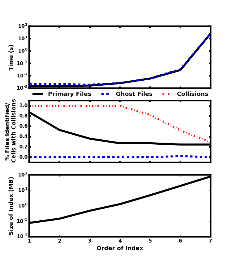
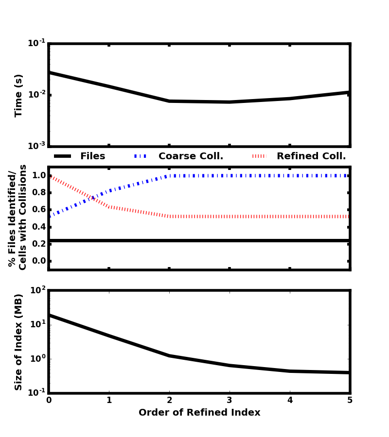
We present a technique for using Morton bitmap indexes to map files and accelerate data analysis.
Theory and Background
Domain Partitioning Between Files
A common analysis task is the selection of data within a subset of the full domain; we use the term "selector" to refer to the selection operator.
If the dataset is split across multiple files, either due to size constraints or to allow for parallel I/O, such selections require every file to be loaded and parsed in order to assemble all of the data within the selection criteria.
This process can be very costly in terms of both the memory required to store the data and the time required to read each file.
However, if the contents of the files are mapped in advanced, only the files touched by the selection will need to be loaded.
This is particularly effective for partitioning schemes that are localized within the domain.
If each file contains data that are localized to one part of the domain, selections of contiguous sub-sections within the domain will require fewer files to be loaded.
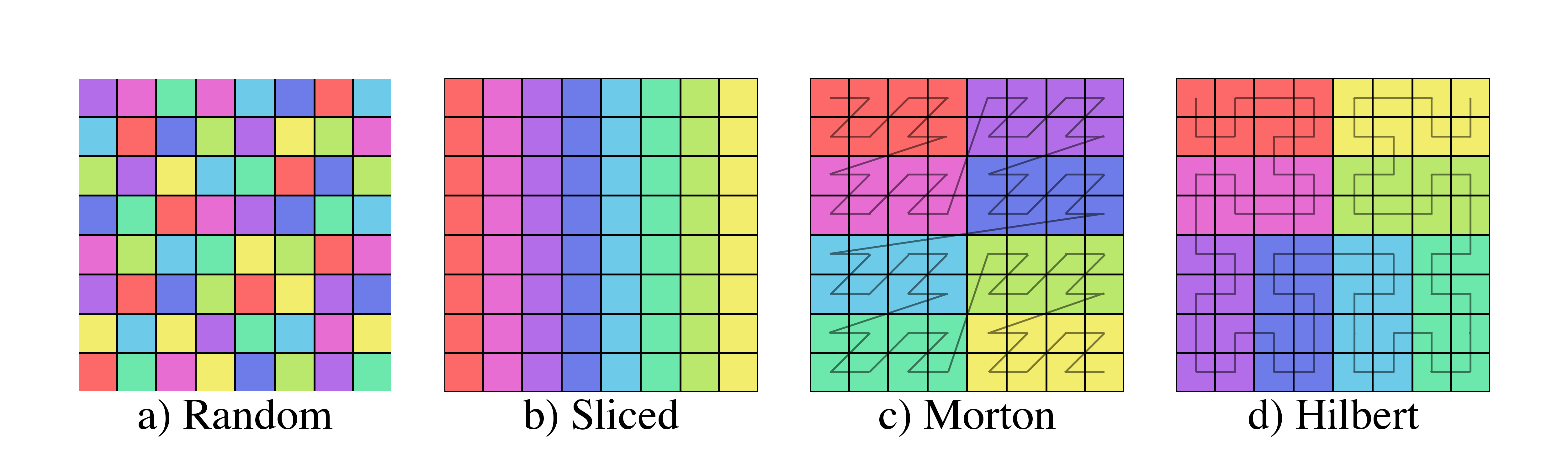
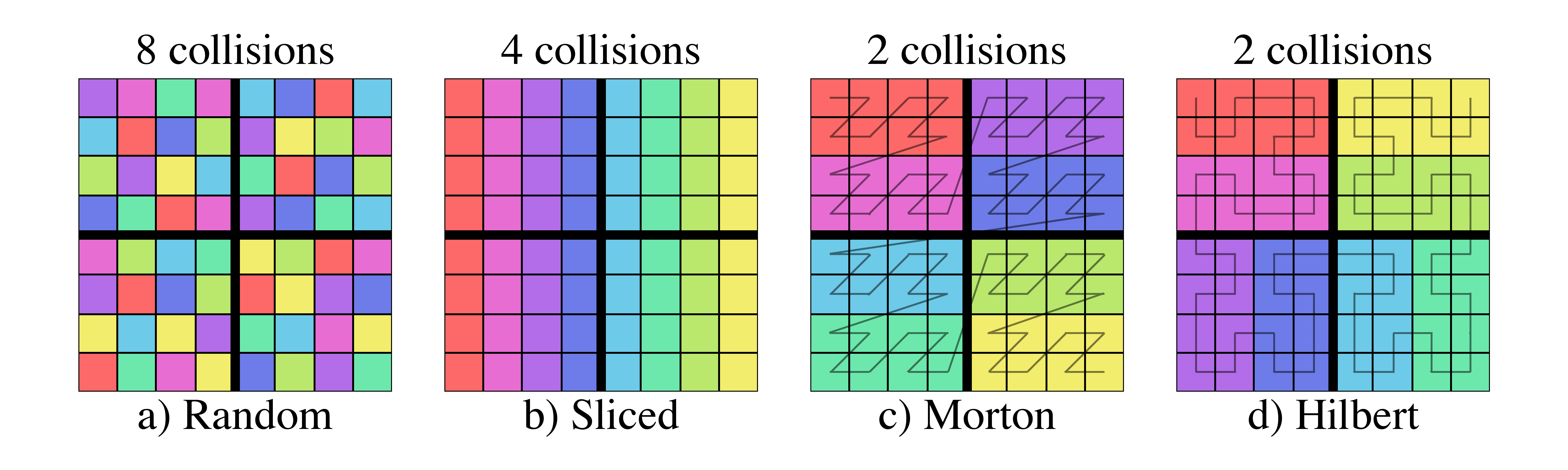
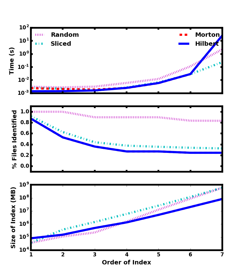
Figure 7 shows four examples of possible partitions of a two-dimensional spatial domain split equally between 8 files.
Figure 7: Examples of four different schemes for partitioning a 2D domain between 8 files.
Each color represents a different file.
Panel (a) is an example where random parts of the domain are contained within each file.
In such a case, many files will need to be loaded for contiguous selections within the domain.
In panel (b), the domain was split between the files along the \(x\) dimension.
Fewer files will need to be loaded for queries along the \(y\)-dimension, but contiguous selection in \(x\) will still require a greater number of files since the partition is not well localized in that dimension.
Panels (c) and (d) are both examples of partitioning the domain between the files along a space filling curve [5,6].
These partitions have the greatest chance of limiting the number of files that must be loaded for a contiguous selection with slightly improved localization for the Hilbert curve.
Consequently, Hilbert curves have also been used for load-balancing in parallel simulation codes like Gadget-2 [7] and RAMSES [8].
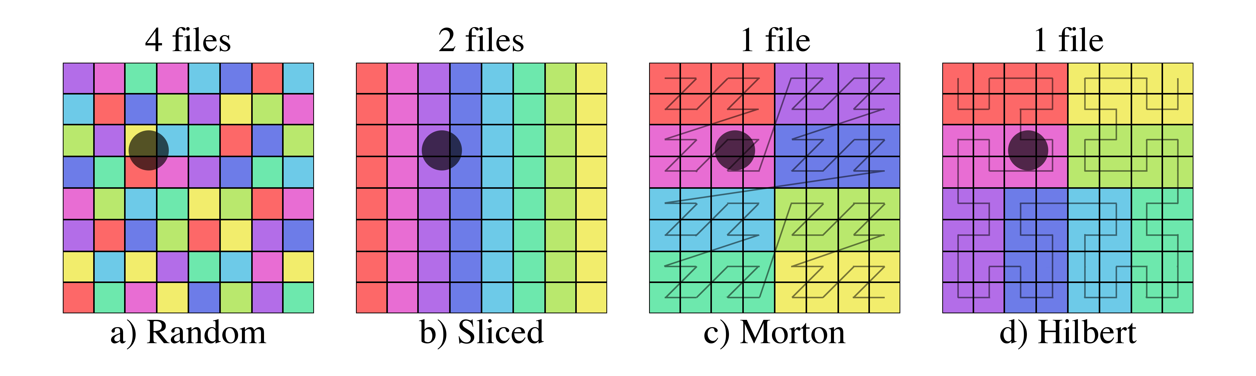
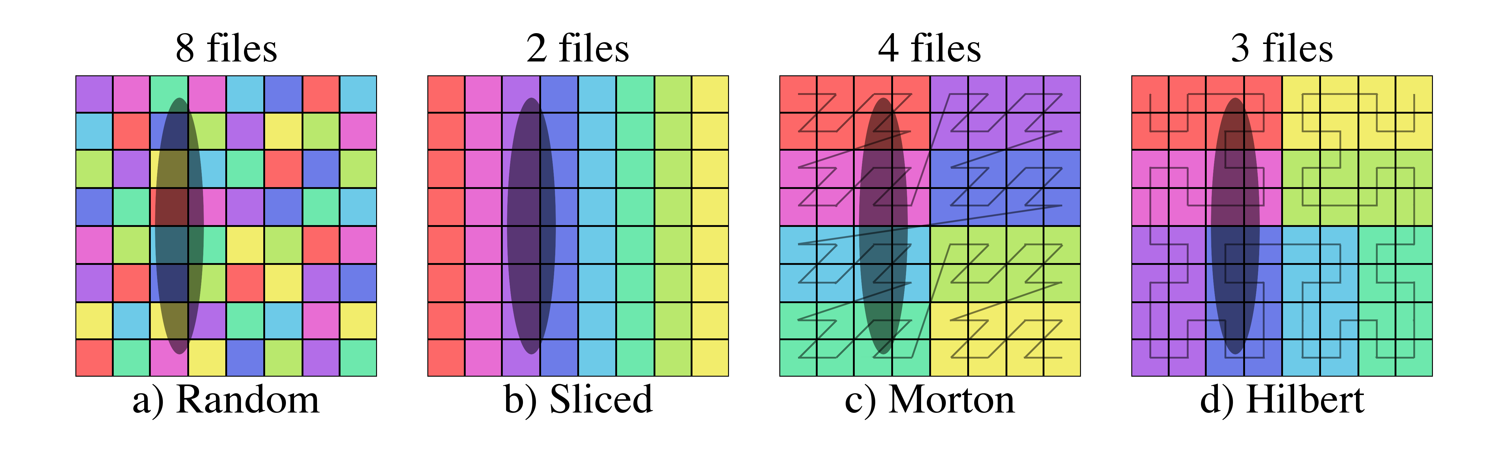
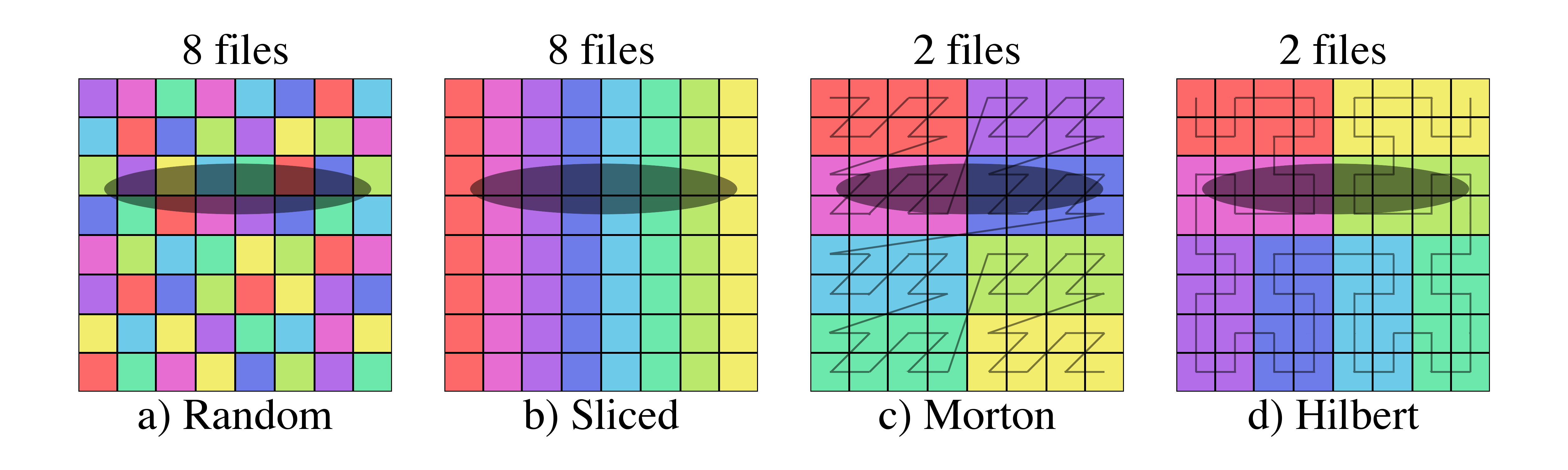
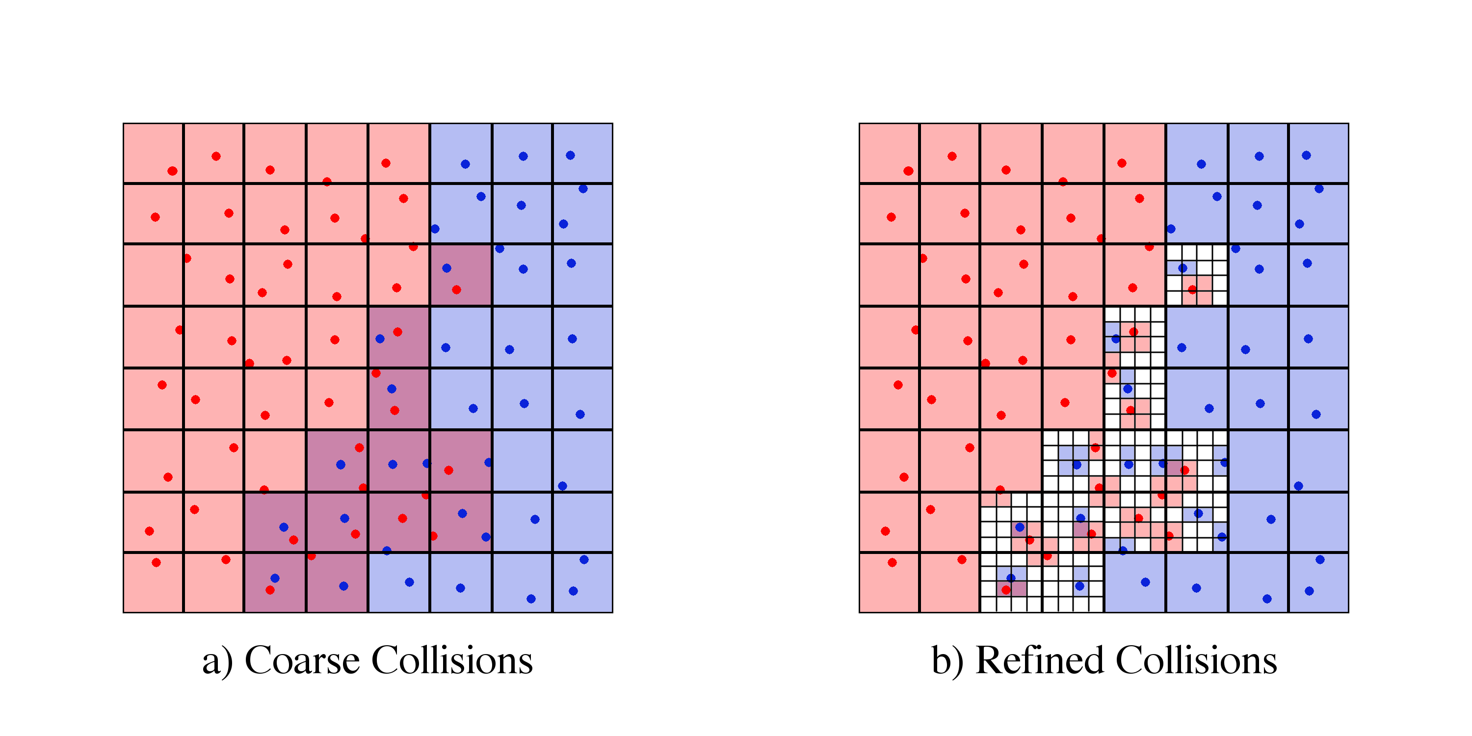
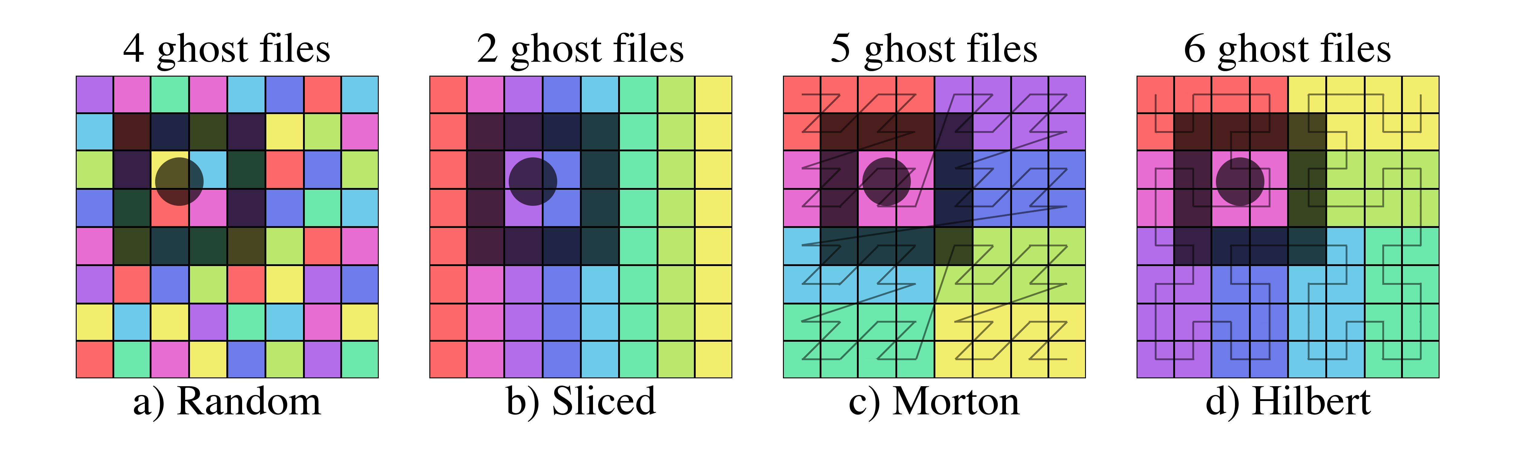
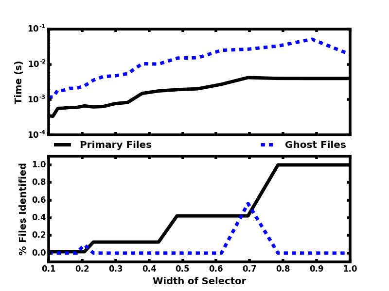
Figure 8 shows examples of three selections within the above domain partitions.
Figure 8: Examples of file selection for four different domain partitions and three different shaded selectors.
The number of files above each images is the number of files that must be loaded in order to get all of the data within the selected region.
Figure 9: Examples of file selection for four different domain partitions and three different shaded selectors.
The number of files above each images is the number of files that must be loaded in order to get all of the data within the selected region.
Figure 10: Examples of file selection for four different domain partitions and three different shaded selectors.
The number of files above each images is the number of files that must be loaded in order to get all of the data within the selected region.
For the smallest selector (first row), the random domain decomposition (a) already requires half of the files to be loaded while more localized schemes require much fewer.
Similarly, while the sliced domain partition (b), requires the fewest files to be loaded when the selector is oriented in the same direction as the slicing (second row), it requires all of the files when the selector is perpendicular to the slicing (third row).
While some datasets may have information on the domain range covered by each file, the partitioning scheme used for simulation output is often decided at runtime, can be system dependent, and may be imperfect.
Files are often partitioned for parallel I/O such that each processor outputs data on the portion of the domain it is responsible for processing.
To limit the cost of communication between processors, the domain will be split across processors such that neighboring processors are responsible for neighboring parts of the domain.
This means that, although the overall partitioning scheme may be known for a given dataset, the exact order of the files will be dependent on the configuration of the processors at runtime.
The partitioning can also be imperfect if the domain decomposition is not perfect at the time of output.
For instance, in astrophysical N-body simulations, it is possible for particles to travel from one processor’s domain to another.
In this case, the partition will only be perfect directly following an update to the domain decomposition.
In cases where the exact file organization is not known or imperfect, it is advantageous to map the files post-process in order to speed up selections for analysis.
Although the same result can be achieved by re-sorting the data itself, creating the map can be less computationally less expensive than re-sorting the data, can be saved for use with multiple selections, and does not required write access; this is typically not feasible, especially in the case of datasets shared by large, distributed communities.
Morton Indices
Morton ordering maps multidimensional data onto a one-dimensional space filling curve [5].
This is done by breaking up the domain into cells where each cell’s position within the \(N\)-dimensional domain can be described by \(N\) integers.
The Morton index of the cell is then created by interleaving the bits of the \(N\) integers to create a single integer that fully describes the cell’s position (see panel (b) Figure 11).
As seen in panel (a) of Figure 11, ordering of the cells by their Morton indices forms a space filling Z-curve.
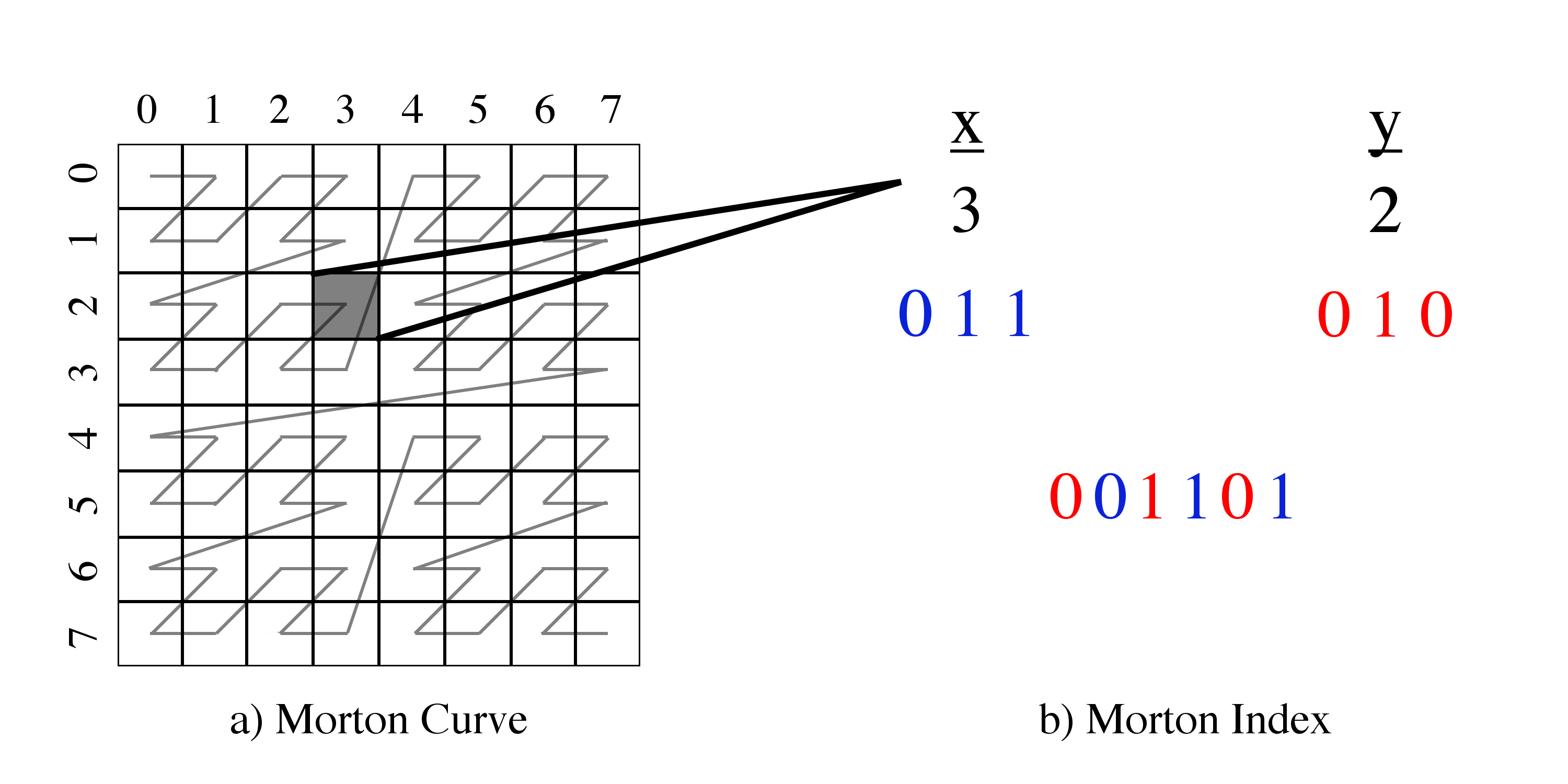
Figure 11: Example of 3rd order Morton curve in two dimensions.
The bits of the \(x\) and \(y\) indices are interleaved to generate a single integer that fully describes the cell’s location within the two-dimensional domain to within \(1/2^{3}\)th of the domain in each dimension.
NOTE: wouldn’t it make more sense to write \(y\) and \(x\) is this order, so that the interleaving could be represented with arrows without crossing them ?
The precision of a single Morton index is only limited by the size of the integer used to store it.
For instance, 64-bit Morton indices in 3 dimensions can be localized to \(1/2^{21}\)th of the domain in each dimension (\(3\times21\) bits = 63 bits).
If the domain is binarily divided into subcells to some order \(k\) in each dimension (i.e.
\(2^{Nk}\) cells), coarser Morton indices can be obtained by simply masking lower bits.
Morton ordering has been used to speed up quadtree construction [9], nearest neighbor searches [10], and range queries [11].
By recording the indices of the cells containing data from each file within a dataset, Morton indices can also be used to construct one-dimensional maps of an \(N\)-dimensional dataset that can be represented as bitmaps.
Bitmaps & EWAH Compression
Bitmap indexes use the values of single bits within an array of bits to describe dataset properties.
This form requires minimal memory and can be filtered using computationally inexpensive boolean operations.
Bitmap indexes have long been popular for use with large data warehouses [12,13,14].
However, as scientific datasets have become larger and more complex, they have also begun to gain traction in a diverse array of scientific fields including geosciences [15], earth sciences TODO: insert citation here ?, rocket science [16,17], high-energy physics [18], and combustion [19].
In cases where data attributes can take on a finite set of values, one bitmap is constructed for each possible attribute value.
Within the bitmap each bit specifies whether or not the corresponding data point has that value.
In this way, queries for data with a single attribute value require consulting only one bitmap and queries of multiple attributes/values can be done using boolean AND operations on the corresponding bitmaps.
In the case of scientific data, which often contains floating point value attributes, the attributes must be binned prior to constructing the bitmaps [20,21,22].
Here, Morton indices are used to bin N-dimensional floating point data onto one-dimension.
As a result, each file can be described by one bitmap.
For each file within a dataset, the Morton indices touched by the data within that file can then be stored in a bitmap index for future searches where the value of bit \(j\) indicates whether or not Morton index \(j\) is touched by the file in question.
For Morton indexing of order \(k\), this would result in a bitmap of length \(2^{Nk}\) bits per file.
For large bitmaps, this can become costly in terms of memory and the time required to perform bitmap operations.
However, Enhanced Word-Aligned Hybrid (EWAH) compression can be used to limit these costs, particularly when the domain is densely or sparsely populated in localized regions [23,24,25].
An EWAH compressed bitmap will be smaller when there are long sequences, or “runs,” of identical values.
This means that an EWAH compressed bitmap will be smallest if either all or none of its bits are set.
An uncompressed bitmap would require the same, maximum, amount of memory in both of these cases.
The locality of Morton indices takes advantage of the EWAH compression.
If there are regions of the domain that are densely/sparsely populated, there Z-order space filling curve ensures that the bits denoting those regions will be adjacent, increasing the likelihood that there will be runs of identical (set/unset) bits and limiting the size of the compressed bitmaps.
Collisions
It is possible that two files will contain data within the same Morton cell.
This would mean that any time that cell is touched by a selection, both files would need to be loaded even if the selection only touches data from one of the files.
Figure 12 provides an example of collisions between two files.
In panel (a) of Figure 12, purple cells are those that contain data from both files, a collision, for a 3rd order Morton index.
Any selector that contained one of those cells would need to load all of the data from both files, even if it only selected part of the cell.
Where the data is highly-concentrated in a central region (for instance, in a galaxy formation simulation with particles centrally-concentrated) this can mean that some regions suffer from worst-case scenario collision.
Figure 12: Examples of a collision between two files.
The red points and blue points are contained by two different files.
The larger grid in both panels denotes the boundaries of 3rd order Morton cells.
The cells containing points from either file are shaded accordingly such that cells containing points from both files are purple.
The smaller grids within these cells on the right are the boundaries of 2nd order Morton cells refining the collisions.
Collisions can be limited by either increasing the order of the index or allowing for multi-resolution indexes [16,17].
Panel (b) of Figure 12 demonstrates an example of nesting a second index within cells that contain collisions.
In those cells which contained collisions, a 2nd order Morton index was added.
Those cells with collisions at the level of the refined index (purple cells in panel (b)) cover a much smaller portion of the domain than the cells with collisions at the level of the coarse index (purple cells in panel (a)).
This means that any given selection is less likely to contain a collision and it will be less likely for a selector to require both files to be loaded unless it actually touches data from both files.
Increasing the order of the coarse index has the same effect as nesting a second refined index within cells with collisions, but can also increases the size of the resulting map and the time it takes to identify files touched by a selection.
However, if the order of the coarse index is too small or the order of the refined index too large, this too can increase the cost of a selection in terms of memory and time.
Section [sec:test_order] discusses this tradeoff and how to choose index orders.
Collisions are more common for file partitioning schemes that are not localized.
Figure 13 shows an example of collisions for the different partitioning schemes discussed in Section [sec:decomp].
Figure 13: Examples of collisions for four different domain partitioning schemes.
The heavy black lines denote 1st order Morton cells.
The presence of more that one file (color) within a Morton cell indicates a collision.
NOTE: from an accessibility standpoint, I must note that using a smooth color gradient may be counter productive for colorblind readers as it makes it a lot harder to perveice that neighbouring regions belong to different files.
For the random domain partition in panel (a), every cell within a 1st order Morton index will contain data from all 8 files.
This means that any selection using a 1st order bitmap index will require every file to be loaded.
For the more localized partitions in panels (c) and (d), only two files touch each Morton cell.
Ghost Zones
It is often the case that, in selecting a region, additional padding around the region should be included in the selection.
This is particularly useful for algorithms that need information about neighboring points in the domain [26,7,27].
For Morton indices, this is straightforward as the indices neighboring Morton cells can be found by incrementing the bits corresponding to each dimension.
We have included the ability to pad selectors with some number of Morton cells referred to as ‘ghost zones’.
Those files that touch ghost zones, but not the selector itself are referred to below as ‘ghost files’.
Depending on how the domain is split between files, the inclusion of ghost zones may or may not increase the number of files that need to be loaded.
Figure 14 shows an example of a ghost zone around the first selector from Figure 8.
Figure 14: Examples of a selector ghost zone with a width of one Morton cell at an index order of 3 for four different domain partitioning schemes.
The shaded circular region is the selector and the shaded box is the ghost zone.
Different partitioning schemes will lead to different numbers of ghost files.
NOTE: same as figure 13
The ghost zone has a width of one Morton cell at an index order of 3 and contains the same part of the domain in each case.
However, due to differences in how the domain was partitioned between the files in the four cases, the number of additional ghost files touched by the ghost zone in each case is different.
This will also depend on the order of the index to which ghost zones are added.
Ghost zones added at the order of the coarse index will be larger than those added at the order of the refined index and will have a higher probability of touching additional files.
While including ghost zones is advantageous when neighbor info is needed, it also increases the computational cost of identifying files (see Section [sec:tests]).
Methods
The basic procedure for constructing the bitmap index is as follows:
Compute coarse indices. For each file in the data set, read in
the data and compute the indices of Morton cells at a given coarse
order that are touched by data contained within that file. These
coarse indices are then stored by setting the corresponding bits in
an EWAH compressed bitmap.
Find collisions. The indices of coarse cells that are touched by
data in more than one file (collisions) are located using bitwise
operations on the file bitmaps. These indices are also stored in an
EWAH compressed bitmap.
Compute refined indices. For each file in the data set, read in
the data and compute the indices of Morton cells at a given refined
order within coarse cells with collisions that are touched by that
file. These refined indices are stored in a map from coarse Morton
index to an EWAH compressed bitmap of refined Morton indices within
that cell.
Output bitmaps. The EWAH compressed bitmaps for the coarse
indices, refined indices, and collisions are saved to an external
index file.
For large datasets and/or high levels of refinement, this can be a time consuming process; however, it must only be done once.
For future selections, the bitmap can be quickly loaded and used to identify files in less time than would be required to load and query each file within the dataset individually.
Selection using a loaded bitmap goes as follows:
Construct selector bitmap. In the same way each file was mapped,
the indices of Morton cells touched by the selector are stored in a
bitmap. This is done by checking for intersection of the selector
with Morton cells at the order of the coarse bitmaps. For contiguous
selectors, this is done at lower order (parent) cells first and
continued recursively until the order of the coarse bitmap is
reached.
If a cell is completely within the selector, all of its child
cells at the coarse order are added to the bitmap.
If a cell intersects the edge of the selector, child cells at
increasing orders are checked until the order of the coarse
bitmaps are reached. If the cell is at the coarse order and
there is a collision between two files, a refined bitmap is the
constructed for the selector in the same manner.
Find files intersecting the selector. Bitwise operations with
the coarse file bitmaps are then used to efficiently identify files
that intersect the selector within coarse cells. If the coarse cells
within the intersection with a file all have collisions with other
files, bitwise operations with the refined file bitmaps are then
used to determine if the file is selected at the order of the
refined index.
If ghost zones are desired, the neighbors of cells that intersect the edge of the selector are added to a separate bitmap.
For cells without collisions, the neighbors are added at the coarse bitmap order.
If there are collisions, the neighbors are added at the refined bitmap order.
Tests
The utility of using Morton index bitmaps for mapping files to decrease query times was tested on artificial N-body simulation datasets containing \(1024^3\) points in three dimensions, distributed between 512 files.
For each test a Morton index bitmap was constructed for the dataset and used to identify files touched by cube shaped three-dimensional selectors.
The performance is assessed in terms of the number of files identified and the average time required to identify them across 10 runs.
If fewer files are touched, fewer files will need to be loaded during analysis of a selected region and the overall fraction of time spent on I/O will be lower.
If less time is required to identify the files touched by a given selector, more selections can be made using the same computational resources.
This was done for varying index orders (Section [sec:test_order]), selector sizes (Section [sec:test_size]), and partitions of the domain between files (Section [sec:test_decomp]).
Index Order
Overall Refinement
The order of the Morton indices used to map the files determines the time required to identify files and the number of collisions that will occur between files.
Higher order indices will result in fewer collisions, but will take longer to query, as seen in Figure 15 Six selectors of varying sizes and positions within the domain where used to identify files based on Morton index bitmaps of varying order.
The test dataset was split across the files using a Hilbert curve of order 6 with 10% scatter between Hilbert cells to simulate an imperfect domain decomposition as can occur if particle positions are updated and output prior to updating the domain decomposition.
Figure 15: Dependence of query time (top), fraction of files selected/cells with collisions (middle), and index size (bottom) on the total refinement of the bitmap index.
The solid black lines correspond to the query times and files identified by just the selectors.
The dashed blue lines correspond to the query times and additional files selected when a ghost zone with the width of one Morton cell is added around the selectors.
The dash-dotted line in the middle panel shows the fraction of cells with collisions between files.
NOTE: maybe this would make more sense as scatter plots ? (connecting dots to fill a continuous yet unreachable space of non-integer-limited x values seems unappropriate.
Below a bitmap index order of 4, there are collisions between multiple files within every cell, resulting in a larger number of files being identified.
However, as the order increases, the number of collisions drops and the file count plateaus at \(\sim25\)%.
This translates to a \(\sim75\)% reduction in the memory and time required for processing files, a significant increase in performance.
For a 7th order bitmap index, selection requires \(>100\times\) the time that the same selection took using a 6th order index, but there is no change in the number of files indicated.
A 6th order index is sufficient to identify the minimal set of files touched by the selectors in this case because the dataset was partitioned between the files along a 6th order Hilbert space filling curve.
While it is generally true that the time required to identify files using a bitmap index will increase exponentially with the size of the index, the order of the index that results in the minimal number of files for any dataset will depend upon how the domain is partitioned between files (see Section [sec:test_decomp]).
The memory required to store the index for the test dataset scales according to \(\propto2^{2k}\), for a \(k^{\mbox{th}}\) order index.
If uncompressed bitmaps had been used instead of EWAH compressed bitmap, the memory would have scaled with the total number of cells contained within the 3-dimensional test domain (\(2^{3k}\)).
Collision Refinement
Increasing the refinement of the primary index does so for the entire domain and, as seen in Section [sec:test_order1], can become costly in terms of the memory required to store the bitmap and the time required to perform operations.
However, it is also possible to increase refinement by nesting a second Morton bitmap index within those cells of the primary index that contain collisions.
As the nested indexes will contain a smaller portion of the domain and data, they will be less complex and can be compressed more efficiently than the primary index covering the entire domain.
This enhanced compression means that, although a greater overall number of EWAH compressed bitmaps will need to be utilized (one for the coarse index and one for each collision within the coarse index), less space will be needed to store the bitmap and bitwise operations will be faster.
Figure 16 shows the results for adding a secondary index of varying order with the overall refinement order of the index (primary index order + secondary index order) held constant at 6.
The test dataset and selectors applied were the same as in Section [sec:test_order1].
Figure 16: Dependence of query time (top), fraction of files selected/cells with collisions (middle), and memory required to store the index (bottom) on the order of the secondary index used to refine collisions.
In the middle panel, the solid black line corresponds with the fraction of files identified, the dash-dotted blue line is the fraction of cells at the first index level that have collisions, and the dotted red line is the fraction of cells at the second index level that have collisions.
When the order of the second refined index is low, the first index is larger resulting in fewer cells with collisions at the first index and more at the second.
The reverse is true when the order of second index is higher.
As the overall order is held constant, the same number of files are identified regardless of the orders of the first and second indexes.
The time required to identify the files is minimized when cells within the first index become saturated with collisions.
For secondary indexes of order 2 or lower, the large increase in performance offered for increases in the index order results from the reduction in the total complexity of the index which translates to shorter times for bitwise operations and less memory required for storage.
Above 2nd order, the overhead from storing and accessing more complex EWAH compressed bitmaps for each collision begins to flatten the memory scaling and increase the time required for queries.
However, selections using higher order secondary indices still require less time than in the case where only a single index is used.
The optimal value for the orders of the first and second indexes will depend upon the dataset in question.
The density of data points within the test dataset used here is relatively uniform throughout the domain and does not need a high level of refinement at collisions.
However, if a datasetwere less uniform with concentrations of points, the optimal order of the second index for performance may be higher.
Selector Size
The time required to identify files touched by a selection will also depend upon the size of the region being selected.
Larger selectors will intersect more indices and more files, resulting in more bitmap operations.
Figure 17 shows the result from varying the selector size.
The same test datasetfrom Section [sec:test_order] was used.
A bitmap index with a 4th order primary Morton index and 2nd order secondary Morton index was used in all cases.
Each cube selector was placed at the center of the domain and scaled along each dimension to some fraction of the total domain.
Figure 17: Dependence of query time (top) and number of files selected (bottom) on selector width in terms of the total domain width.
The solid black lines correspond to the query times and files identified by the selectors alone.
The dashed blue lines correspond the query times and additional files identified when a ghost zone with a width of one cell is added to the selector.
As the selector increases in size, it touches a greater number of files, resulting in longer query times.
The number of files touched increases in steps due to the way the test dataset was partitioned between files.
Using the Hilbert curve, the domain covered by any one file is localized and will have a rectangular shape.
This results in an ordered structure that is similar along all dimensions.
An increase in the number of files touched indicates that the selector has grown past a file boundary in all directions.
It is just prior to these jumps that ghost files are present.
If the selector edge is near a file boundary, ghost zones have the potential to overlap the domains contained by neighboring files that are not already touched by the selector.
For such a highly ordered dataset, the ghost zones will only identify additional files for selectors that are nearing the edges of file boundaries.
However, queries including ghost zones require slightly more time even when this is not the case.
Domain Partitioning
As discussed in Section [sec:decomp], a bitmap index is more effective in cases where the domain is partitioned between files in a localized way.
If files contain non-contiguous parts of the domain, contiguous selections will require more files to be loaded.
Figure 18 shows results for four different partitioning schemes.
All four data sets cover the same three-dimensional domain with \(1024^3\) points split across 512 files.
The Hilbert dataset is the same one used in previous tests (see Section [sec:test_order] for a description).
The Morton dataset is constructed in a similar way to the Hilbert dataset with file partitions occurring along a 6th order Morton curve and including a 10% scatter of points between Morton cells.
The sliced dataset is partitioned in slices along one dimension with 10% scatter of points between adjacent slices.
Files in the random dataset contain a random sample of points, uniformly distributed across the domain.
Figure 18: Dependence of query time (top), the number of files selected (middle), and the size of the index (bottom) on index order for different domain partitioning between files.
The dotted magenta lines are for a randomly partitioned dataset, the cyan dashed-dotted lines are a dataset partitioned by equal slices alone one dimension, the dashed red lines are a dataset partitioned along an 6th order Morton curve, and the solid blue lines are a dataset partitioned along a 6th order Hilbert curve.
NOTE: it looks like the Morton curve is almost always behind the Hilbert one. Can you use zorder to put it at the frontrow instead so that we can see both ?
Many more files are identified for the random dataset than those datasets with localized partitioning of the domain.
Above an order of 3, very few files could be excluded for the random dataset.
This was not true for the localized partitioning schemes.
At the highest order, only \(\sim20-30\)% of the files within these datasets would need to be loaded in order to get all of the data within the selected regions, while \(\sim80\)% of the files in the random dataset would be required.
The smallest fraction of files were identified for the Hilbert and Morton datasets, with a slightly greater fraction being identified for the sliced dataset.
For a 6th order index and below, queries on the Morton and Hilbert partitioned datasets are the fastest.
An index order of 7 provides refinement beyond the 6th order curves used to partition the dataset between the files and the required for queries on these datasets increases dramatically.
The sliced dataset performed particularly well in this case because the selectors used were cubes and did not preferentially select along any one dimension.
Overall, this technique offers a considerable improvement in performance over other methods that require reading, evaluating and discarding all of the particles.
Summary & Discussion
Mapping files using Morton bitmap indexes speeds up analysis of large datasets split across multiple files by reducing the number of files that need to be loaded in order to perform operations on a subset of the full domain.
The time required for making selections using the bitmap index is minimal for even large datasets and can be optimized by partitioning the domain between files in a localized way and using an index or indexes of appropriate order for the dataset.
Without an index, queries require loading the data contained in every file into memory and then searching the data for those points that are selected by the query.
With a bitmap index, queries require loading the index, using it to identify the files touched by the query, reading in the data contained within the identified files, and searching the data for points selected by the query.
In this way, the bitmap index can decrease the computational cost of reading in the data and selecting data points if it identifies a subset of the total number of files.
While using an existing bitmap index decreases the time required for queries in this case, constructing a bitmap index can be more computationally expensive than directly querying the data without a bitmap index.
Therefore, in the case where only a small number of selections need to be made, it will be more efficient to perform direct queries of the data than to construct and utilize the bitmap index.
Bitmap indexing is particularly useful in astronomy and astrophysics.
Output from N-body simulations is often split between multiple files to take advantage of parallel I/O and the domain decomposition generally leads to localized partitioning between files [7,27,28].
Currently, this technique is most useful for datasets split across multiple files.
However, it can also be applied to single files by dividing the file’s contents into chunks.
As in the multi-file case, the single file would need to be organized such that chunks were localized within the domain to take full advantage of the bitmaps.
In addition, while the current implementation of this method is designed for three-dimensional spatial datasets like those produced by astrophysical simulations, the same methods can be applied to non-spatial datasets with arbitrary dimensionality.
Code
These procedures have been implemented as part of the yt Python package [29] in order to facilitate the analysis of large astrophysical N-body simulations; currently undergoing review for inclusion in a future version of yt (4.0 or later), our implementation is available at https://bitbucket.org/langmm/yt-bitmap.
NOTE: This use to say “3.4 or later”. Now it’s pretty clear this section is a bit dated. Hasn’t the bitmap stuff been merged by now ?
The open source EWAHBoolArray C++ package is used for implementing EWAH bitmaps [24,25] and exposed to Python using Cython [30].
Acknowledgment
The authors would like to thank Daniel Lemire for his open source EWAH implementation.
yt is developed by a large number of independent researchers from numerous institutions around the world.
Their commitment to open science has helped make this work possible.
Visualization and Volume Rendering
The primary method by which researchers interact with their data in yt is via visualization; from the standpoint of the library, however, this is a side-effect of the various analysis, regularization and data-processing algorithms that are implemented within yt.
Nearly all of the visualization that is done using yt utilizes the matplotlib library for actual deposition of pixels into an image format, although all of the input to that deposition is conducted by yt.
Making this distinction is important, because it underscores the relationship between the different libraries and how they exist in the ecosystem of scientific software; yt does not replace matplotlib, but rather, augments it by providing a grammar of analysis of volumetric data and defining how that grammar is translated into visual representations as presented by matplotlib.
CC: discuss ray traversal for patch-based datasets + oct-based datasets.
Pixelizing Variable-Mesh Objects
The results of either projecting or slicing through a logically-cartesian finite volume dataset is represented in yt as a collection of pixel positions and widths.
These objects, hereafter referred to as exposing the “variable mesh” interface (as originated in HippoDraw), are not typically suitable for direct visualization.
Many visualization libraries, including matplotlib, would necessarily regard these as collections of patches of fixed size, supplying them to the underlying engine.
To optimize for repeated rendering, yt provides its own “pixelization” routines that take advantage of the input data structures.
These “pixelizers” (or “rasterizers”) can account for periodic data, variable resolution, overlapping and disjoint datasets, and non-Cartesian coordinate systems.
The pixelizers in yt are implemented in Cython, and they accept an input “image plane” buffer (with extent) as well as the variable mesh to be deposited.
Pixelizers exist for cartesian coordinates, cylindrical and spherical coordinates, off-axis cartesian planes, and for the Mollweide orthographic projection.
Each of these pixelizers follows a roughly identical process for depositing source pixels into the image plane.
The outer loop is over the input pixels, \(p_i\), composed of \(x_i, y_i, dx_i, dy_i, v_i\), where \(x\) and \(y\) refer to the coordinate system; in practice this means they may actually represent the \(r\), \(\theta\), \(\phi\) or other coordinates.
Compute left and right edges of the bounding box for this pixel in the resolution of the image plane
Iterate over the first image plane coordinate from the left edge to the right edge of the bounding box
Iterate over the second image plane coordinate from the left edge to the right edge of the bounding box
Map from the coordinate system to the image plane and deposit \(v\)
In practice, this is a fast operation, as long as the inner loops are sufficiently well determined; for instance, when depositing an input pixel with a width of \(w\) into an image plane where the pixel width corresponds to a width of \(w/16\), only \(16^2\) pixels (with a high-degree of sequential ordering) have to be iterated over.
The spherical and cylindrical pixelization routines operate similarly, but are somewhat degraded by a lower degree of locality in the final mapping from coordinate system to image plane.
Recent work has been done to port the pixelization routines to Rust and compiling these to WebAssembly, resulting in the development of the Widgyts project.
Widgyts provides a browser-side Jupyterlab interface to the pixelization routines, enabling extremely low-latency exploration of datasets.
Higher-Order Unstructured Mesh Elements
Software Volume Rendering
The volume rendering is based on classical concepts for rendering 3D objects, and relies on the notion of a scene, a camera and an object to render.
The object to render can be any data container of supported AMR datasets (either patch-based and octree-based datasets).
The implementation of the volume rendering is based on integrating a transfer function along the direction of ray.
Patch-based ray traversal
TODO
Octree ray traversal
Casting rays through an octree can be achieved efficiently by relying on the octree structure.
In order to abstract away the underlying layout of the data, we first construct an octree that contains all leaf cells in the data container.
We store all cells as octs with no children, and mark them with their position within the data container, going from \(0\) to \(N_\mathrm{cell}-1\).
Octs that are inserted in the process of building the tree are not marked nor indexed.
We also compute the vertex-centered data for all cells in the container.
Note that, contrary to the octree utilized to index the data from octree datasets, this octree may span multiple domains and contains all levels from the root level (that contains a single oct the size of the simulation domain) all the way down to the leaf cells.
We then cast rays off the camera, and for each ray, we compute the ordered list of the \(N\) cells it intersects with together with the intersection points along the ray [31].
In the following, we will write the coordinate along the ray as \(t\), with the camera located at \(t=0\).
In general the tree may contain holes (this may happen if the data container is a region selector), so that the exit coordinate out of a cell may not coincide with the entry coordinate through the next cell. In practice, we solve this by storing for each cell both the entry and exit coordinates of the ray.
The algorithm relies on the fact that if a ray passes through an oct and intersects with its six faces at coordinate along the ray \(t_{xi}, t_{yi}, t_{zi}\) (on entry) and \(t_{xo}, t_{yo}, t_{zo}\) (on exit), then its intersection with the inner cells’ faces can be computed explicitly from these six values and their half point \((t_{xi}+t_{xo})/2, (t_{yi}+t_{yo})/2, (t_{zi}+t_{zo})/2\). This implies that each call to the algorithm only need computing one division and a few simple arithmetic comparisons.
It also uses the fact that for a given oct, we can compute which cell the ray will intersect with first, and from any given cell, which cell the the ray will intersect next.
The algorithm then works as follows. If the ray does not intersect with the root oct, then the algorithm returns an empty list of cell crossed and \(t\) values.
Otherwise, initialize an empty list of cells traversed and \(t\)-values. a) Find the intersection of the ray with all six faces of the oct. b) If the current oct is marked, store the entry and exit \(t\)-values and the index of the oct in their respective list and return. c) If the current oct is not marked, find the first cell the ray intersects with and call the algorithm recursively (starting at step a) with the oct contained in the cell, if any). d) Find the next cell within the oct. If there is no next cell, return. Otherwise, call the algorithm recursively (starting at step a) with the oct contained in the cell, if any) then go back to d).
On exit of the algorithm, we then have a list of cells and \(t\)-values.
For each cell in the list, we then call the sampler with the vertex-centered values and the entry and exit coordinates.
An example of the volume rendering of a galaxy in a zoom-in cosmological simulation made with RAMSES is shown on Figure 19.
Figure 19: Volume rendering of gas density isocontours around a galaxy in a cosmological zoom-in simulation performed with RAMSES. Adapted from [32].
Sampling functions
TODO
Hardware-accelerated Volume Rendering
Units and Quantities
At a basic level, yt is an engine for converting data dumped to disk by a simulation code into a physically meaningful result.
Attaching units to simulation data makes it possible to perform dimensional analysis on the simulation data, adding additional opportunities for catching errors in a data processing pipeline.
In addition, it becomes straightforward to convert data from one unit system to another.
In yt 3.0 we handle units in a an automatic fashion, leveraging the symbolic math library sympy.
Instead of returning a NumPy ndarray when users query yt data objects for fields, return a YTArray, a subclass of ndarray.
YTArray preserves ndarray’s array operations, including deep and shallow copies, broadcasting, and views.
Augmenting ndarray, YTArray attaches unit metadata to the array data, enabling runtime checking of unit consistency in arithmetic operations between YTArray instances, and making it trivial to compose new units using algebraic operations.
As a trivial example, when one queries a data object (here given the generic name dd) for the density field, we get back a YTArray, including both the simulation data for the density field, and the units of the density field, in this case \(\rm{g}/\rm{cm}^3\):
YTArray is primarily useful for attaching units to NumPy ndarray instances.
For scalar data, we have created the new YTQuantity class.
YTQuantity is a subclass of YTArray with the requirement that the “array data” associated with the instance be limited to one element.
YTQuantity is primarily useful for physical constants and ensures that the units are propagated correctly when composing quantities from arrays, physical constants, and unitless scalars:
If a user needs the field in a different unit system, they can quickly convert using convert_to_units or in_units.
When a Dataset object is instantiated, it will its self instantiate and set up a UnitRegistry class that contains a full set of units that are defined for the simulation. This registry includes both concrete physical units like cm or K but also units symbols that correspond to the unit system used internally in the simulation.
The new unit systems lets us to encode the simulation coordinate system and scaling to physical coordinates directly into the unit system. We do this via “code units”.
Every Dataset has a length_unit, time_unit, and mass_unit, attribute that the user can quickly and easily query to discover the base units of the simulation. For example:
>>>import yt>>> ds = yt.load("Enzo_64/DD0043/data0043")>>>print(ds.length_unit)128 Mpccm/h>>>print(ds.quan(1.0, "code_length").in_units("Mpccm/h"))128 Mpccm/h>>>print(ds.length_unit.in_cgs())5.55517285026e+26 cm
Optionally velocity_unit, pressure_unit, temperature_unit, and density_unit may be defined as well if the units for these fields cannot be inferred from the mass, length, and time units.
Additionally, we allow conversions to the simulation unit system.
Data in code units are available by converting to code_length, code_mass, code_time, code_velocity, code_density, code_magnetic, code_pressure, code_metallicity, or any combination of those units.
Code units preserve dimensionality: an array or quantity that has units of cm will be convertible to code_length, but not to code_mass.
On-disk data are also be available to the user, presented in unconverted code units.
To obtain on-disk data, a user need only query a data object using an on-disk field name:
Here, the first data object query is returned in code units, while the second is returned in CGS units.
This is because ("enzo", "Density") is an on-disk field, while ("gas", "density") is an internal yt field.
Implementation}
Our unit system has 6 base dimensions, mass, length, time, temperature, and angle.
The unitless dimensionless dimension, which we use to represent scalars is also technically a base dimension, although a trivial one.
For convenience, we also create dimensionless unit symbols to represent quantities like metallicity that are formally dimensionless, but it is convenient to represent in a unit system.
For each dimension, we choose a base unit.
Our system’s base units are grams, centimeters, seconds, Kelvin, and radian.
All units can be described as combinations of these base dimensions along with a conversion factor to equivalent base units.
The choice of CGS as the base unit system is somewhat arbitrary.
Most unit systems choose SI as the reference unit system.
We use CGS to stay consistent with the rest of the yt codebase and to reflect the standard practice in astrophysics.
In any case, using a physical coordinate system makes it possible to compare quantities and arrays produced by different datasets, possibly with different conversion factors to CGS and to code units.
We go into more detail on this point below.
In the future, we plan to make the preferred internal coordinate system a user-configurable option.
We provide sympy Symbol objects for the base dimensions.
The dimensionality of all other units should be sympyExpr objects made up of the base dimension objects and the sympy operation objects Mul and Pow.
Let’s use some common units as examples: gram (g), erg (erg), and solar mass per cubic megaparsec (Msun / Mpc\(^3\)).
g is an atomic, CGS base unit, erg is an atomic unit in CGS, but is not a base unit, and Msun/Mpc\(^3\) is a combination of atomic units, which are not in CGS, and one of them even has an SI prefix.
The dimensions of g are mass and the cgs factor is 1.
The dimensions of erg are mass * length$^2$ * time\(^{-2}\) and the cgs factor is 1.
The dimensions of Msun/Mpc\(^3\) are mass / length\(^3\) and the cgs factor is about 6.8e-41.
We use the UnitRegistry class to define all valid atomic units.
All unit registries contain a unit symbol lookup table (dict) containing the valid units’ dimensionality and cgs conversion factor.
Here is what it would look like with the above units:
Note that we only define atomic units here.
There should be no operations in the registry symbol strings.
When we parse non-atomic units like Msun/Mpc**3, we use the registry to look up the symbols.
The unit system in yt knows how to handle units like Mpc by looking up unit symbols with and without prefixes and modify the conversion factor appropriately.
We construct a Unit object by providing a string containing atomic unit symbols, combined with operations in Python syntax, and the registry those atomic unit symbols are defined in.
We use sympy’s string parsing features to create the unit expression from the user-provided string.
Unit objects are associated with four instance members, a unit Expression object, a dimensionality Expression object, a UnitRegistry instance, and a scalar conversion factor to CGS units.
These data are available for a Unit object by accessing the expr, dimensions, registry, and cgs_value attributes, respectively.
Unit provides the methods same_dimensions_as, which returns True if passed a Unit object that has equivalent dimensions, get_cgs_equivalent, which returns the equivalent cgs base units of the Unit, and the is_code_unit property, which is True if the unit is composed purely of code units and False otherwise.
Unit also defines the mul, div, pow, and eq operations with other unit objects, making it easy to compose compound units algebraically.
The UnitRegistry class provides the add, remove, and modify methods which allows users to add, remove, and modify atomic unit definitions present in UnitRegistry objects.
A dictionary lookup table is also attached to the UnitRegistry object, providing an interface to look up unit symbols.
In general, unit registries should only be adjusted inside of a code frontend, since otherwise quantities and arrays might be created with inconsistent unit metadata.
Once a unit object is created, it will not receive updates if the original unit registry is modified.
Creating YTArray and YTQuantity instances
There are two ways to create new array and quantity objects: via a constructor, and by multiplying scalar data by a unit quantity.
Class Constructor
The primary internal interface for creating new arrays and quantities is through the class constructor for YTArray.
The constructor takes three arguments.
The first argument is the input scalar data, which can be an integer, float, list, or array.
The second argument, input_units, is a unit specification which must be a string or Unit instance.
Last, users may optionally supply a UnitRegistry instance, which will be attached to the array.
If no UnitRegistry is supplied, a default unit registry is used instead.
Unit specification strings must be algebraic combinations of unit symbol names, using standard Python mathematical syntax (i.e.
** for the power function, not ^).
In addition to the class constructor, we have also defined two convenience functions, quan, and arr, for quantity and array creation that are attached to the Dataset base class.
These were added to syntactically simplify the creation of arrays with the UnitRegistry instance associated with a dataset.
These functions work exactly like the YTArray and YTQuantity constructors, but pass the UnitRegistry instance attached to the dataset to the underlying constructor call.
For example:
This example illustrates that the array is being created using ds.unit_registry, rather than the default_unit_registry, for which code_length is equivalent to cm.
Multiplication
New YTArray and YTQuantity instances can also be created by multiplying YTArray or YTQuantity instances by float or ndarray instances.
To make it easier to create arrays using this mechanism, we have populated the yt.units namespace with predefined YTQuantity instances that correspond to common unit symbol names.
For example:
>>>from yt.units import meter, gram, kilogram, second, joule >>> kilogram * meter**2== joule True>>>from yt.units import m, kg, s, W >>> kg*m**2/s**3== WTrue>>>from yt.units import kilometer >>> three_kilometers =3*kilometer >>>print(three_kilometers)3.0 km>>>from yt.units import gram, kilogram >>>print(gram+kilogram)1001.0 g >>>print(kilogram+gram)1.001 kg >>>print(kilogram/gram)1000.0 dimensionless
Handling code units
Code units are tightly coupled to on-disk parameters.
To handle this fact of life, the yt unit system can modify, add, and remove unit symbols via the UnitRegistry.
Associating arrays with a coordinate system
To create quantities and arrays in units defined by a simulation coordinate system, we associate a UnitRegistry instance with Dataset instances.
This unit registry contains the metadata necessary to convert the array to CGS from some other known unit system and is available via the unit_registry attribute that is attached to all Dataset instances.
We have modified the definition for set_code_units in the StaticOutput base class.
In this new implementation, the predefined code_mass, code_length, code_time, and code_velocity symbols are adjusted to the appropriate values and length_unit, time_unit, mass_unit, velocity_unit attributes are attached to the StaticOutput instance.
If there are frontend specific code units they should also be defined in subclasses by extending this function.
Mixing modified unit registries
It becomes necessary to consider mixing unit registries whenever data needs to be compared between disparate datasets.
The most straightforward example where this comes up is a cosmological simulation time series, where the code units evolve with time.
The problem is quite general — we want to be able to compare any two datasets, even if they are unrelated.
We have designed the unit system to refer to a physical coordinate system based on CGS conversion factors.
This means that operations on quantities with different unit registries will always agree since the final calculation is always performed in CGS.
The examples below illustrate the consistency of this choice:
For the last two examples, the answer is not the seemingly trivial \(128^2=16384,\rm{Mpccm}^2/h^2\).
This is because the new quantity returned by the multiplication operation inherits the unit registry from the left object in binary operations.
This convention is enforced for all binary operations on two YTarray objects.
Results are always consistent when referencing an unambiguous physical coordinate system:
If we detect that we are loading a cosmological simulation performed in comoving coordinates, extra comoving units are added to the dataset’s unit registry.
Comoving length unit symbols are still named following the pattern <length symbol>cm, i.e.
Mpccm.
The \(h\) symbol is treated as a base unit, h, which defaults to unity.
The Dataset.set_units updates the h symbol to the correct value when loading a cosmological simulation.
User-Friendliness
Publication-Ready Figures
Jupyter Integration
Halo-Finding and Catalogs
Scaling and Parallelism
Performance of Operations
Inline Analysis
Simple Parallelism
Analysis Modules
Extensions and Ecosystem
Trident
Trident [33] is a Python-based open-source tool for post-processing hydrodynamical simulations to produce synthetic absorption spectra and related data.
In many ways, Trident is the first external package that utilizes yt to provide data access and numerical operations, but then builds on those to develop detailed, astrophysically-aware systems for processing and analyzing that data.
Building on yt for access to halo catalogs, and implementing a similar system for derived fields as applied to graph datasets, ytree [35] is a system for analyzing merger trees from analysis of dark matter halos in cosmological simulations.
ytree provides flexibility in determining the path that a given analysis takes through the graph of merger trees; for instance, it enables the user to select if they wish to follow the “most massive” progenitor halo backwards in time, or even to set their own criteria for this.
Connecting this to the raw, unprocessed data from the simulation (such as the unsampled particle or cell content that comprises the halos) allows researchers to deepen and guide their analysis based on the physical characteristics of the merger history.
2. yt: A MULTI-CODE ANALYSIS TOOLKIT FOR ASTROPHYSICAL SIMULATION DATA
Matthew J. Turk, Britton D. Smith, Jeffrey S. Oishi, Stephen Skory, Samuel W. Skillman, Tom Abel, Michael L. Norman The Astrophysical Journal Supplement Series (2011-01-01) https://doi.org/ft6md2
DOI: 10.1088/0067-0049/192/1/9
4. The LSST Data Management System
Mario Jurić, Jeffrey Kantor, K-T Lim, Robert H. Lupton, Gregory Dubois-Felsmann, Tim Jenness, Tim S. Axelrod, Jovan Aleksić, Roberta A. Allsman, Yusra AlSayyad, … LSST Project eprint arXiv:1512.07914 (2015) http://adsabs.harvard.edu/abs/2015arXiv151207914J
5. A computer oriented geodetic data base and a new technique in file sequencing
G. M. Morton IBM Ltd. (1996)
32. Gravitational torques dominate the dynamics of angular momentum of the accreted gas at $z>2$
Corentin Cadiou, Yohan Dubois, Christophe Pichon in prep.
33. Trident: A Universal Tool for Generating Synthetic Absorption Spectra from Astrophysical Simulations
Cameron B. Hummels, Britton D. Smith, Devin W. Silvia The Astrophysical Journal (2017-09-20) https://doi.org/gcx4th
DOI: 10.3847/1538-4357/aa7e2d
34. The formation of submillimetre-bright galaxies from gas infall over a billion years
Desika Narayanan, Matthew Turk, Robert Feldmann, Thomas Robitaille, Philip Hopkins, Robert Thompson, Christopher Hayward, David Ball, Claude-André Faucher-Giguère, Dušan Kereš Nature (2015-09-23) https://doi.org/f7r445
DOI: 10.1038/nature15383 · PMID: 26399829
The authors of this paper would like to extend their deepest gratitude to the many, many individual and institutions that have contributed, directly or indirectly, to the growth of both yt and the yt community.
We particularly thank KIPAC and SLAC at Stanford, the University of California at San Diego and Santa Cruz, the High-Performance Astro Computing Center, Columbia University, the University of Illinois, University of Colorado at Boulder, University of Edinburgh, the scientific Python community, NumFOCUS,
 XXXX-XXXX-XXXX-XXXX
·
XXXX-XXXX-XXXX-XXXX
·  yt-project
·
yt-project
·  yt_astro